SPLINE

1. SPLINE Spline

2. Outline • Spline History • Bezier Curve • Bezier Basis and Geometry Matrice • Bezier Blending Function • B-Spline Curve • B-Spline Uniform • Nonuniform, Rational, B-Spline (NURBS) • Converting Between Spline Spline

3. Splines - History • Draftsman use ‘ducks’ and strips of wood (splines) to draw curves • Wood splines have second-order continuity • And pass through the control points A Duck (weight) Ducks trace out curve Spline

4. Bézier Curves (1/2) • Similar to Hermite, but more intuitive definition of endpoint derivatives • Four control points, two of which are knots Spline

5. Bézier Curves (2/2) • The derivative values of the Bezier Curve at the knots are dependent on the adjacent points • The scalar 3 was selected just for this curve Spline

6. Bézier vs. Hermite • We can write our Bezier in terms of Hermite • Note this is just matrix form of previous equations • Now substitute this in for previous Hermite Spline

7. Bézier Basis and Geometry Matrices • Matrix Form Spline

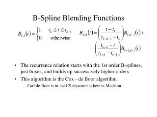
8. Bézier Blending Functions • Look at the blending functions • This family of polynomials is called order-3 Bernstein Polynomials • C(3, k) tk (1-t)3-k; 0<= k <= 3 • They are all positive in interval [0,1] • Their sum is equal to 1 • Thus, every point on curve is linear combination of the control points • The weights of the combination are all positive • The sum of the weights is 1 • Therefore, the curve is a convex combination of the control points Spline

9. Why more spline slides? • Bezier and Hermite splines have global influence • Piecewise Bezier or Hermite don’t enforce derivative continuity at join points • Moving one control point affects the entire curve • B-splines consist of curve segments whose polynomial coefficients depend on just a few control points • Local control Spline

10. p2 p6 p1 Q4 Q5 Q3 Q6 p3 p0 p4 p5 B-Spline Curve • Start with a sequence of control points • Select four from middle of sequence (pi-2, pi-1, pi, pi+1) d • Bezier and Hermite goes between pi-2 and pi+1 • B-Spline doesn’t interpolate (touch) any of them but approximates the going through pi-1 and pi Spline

11. Uniform B-Splines • Approximating Splines • Approximates n+1 control points • P0, P1, …, Pn, n ¸ 3 • Curve consists of n –2 cubic polynomial segments • Q3, Q4, … Qn • t varies along B-spline as Qi: ti <= t < ti+1 • ti (i =integer)are knot points that join segment Qi-1 to Qi • Curve is uniform because knots are spaced at equal intervals of parameter,t • First curve segment, Q3, is defined by first four control points • Last curve segment, Qm, is defined by last four control points, Pm-3, Pm-2, Pm-1, Pm • Each control point affects four curve segments Spline

12. B-spline Basis Matrix • Formulate 16 equations to solve the 16 unknowns • The 16 equations enforce the C0, C1, and C2 continuity between adjoining segments, Q Spline

13. B-Spline Basis Matrix • Note the order of the rows in my MB-Spline is different from in the book • Observe also that the order in which I number the points is different • Therefore my matrix aligns with the book’s matrix if you reorder the points, and thus reorder the rows of the matrix Spline

14. B-Spline (1/2) • Points along B-Spline are computed just as with Bezier Curves Spline

15. B-Spline (2/2) • By far the most popular spline used C0, C1, and C2 continuous • Locality of points Spline

16. Nonuniform, Rational B-Splines(NURBS) • The native geometry element in Maya • Models are composed of surfaces defined by NURBS, not polygons • NURBS are smooth • NURBS require effort to make non-smooth Spline

17. What is a NURB? • Nonuniform: The amount of parameter, t, that is used to model each curve segment varies • Nonuniformity permits either C2, C1, or C0 continuity at join points between curve segments • Nonuniformity permits control points to be added to middle of curve Spline

18. What do we get? • NURBs are invariant under rotation, scaling, translation, and perspective transformations of the control points (nonrational curves are not preserved under perspective projection) • This means you can transform the control points and redraw the curve using the transformed points • If this weren’t true you’d have to sample curve to many points and transform each point individually • B-spline is preserved under affine transformations, but that is all Spline

19. Converting Between Splines • Consider two spline basis formulations for two spline types • We can transform the control points from one spline basis to another • With this conversion, we can convert a B-Spline into a Bezier Spline • Bezier Splines are easy to render Spline

20. Rendering Splines • Horner’s Method • Incremental (Forward Difference) Method • Subdivision Methods Spline

21. Horner’s Method • Three multiplications • Three additions Spline

22. Forward Difference • But this still is expensive to compute • Solve for change at k (Dk) and change at k+1 (Dk+1) • Boot strap with initial values for x0, D0, and D1 • Compute x3 by adding x0 + D0 + D1 Spline

23. Subdivision Methods Spline

24. Referensi • .Hill, Jr., COMPUTER GRAPHICS – Using Open GL, Second Edition, Prentice Hall, 2001 • ___________, Interactive Computer Graphic, Slide-Presentation, (folder : Lect_IC_AC_UK) • ­­­­­­­­­­­­­­­­­­Michael McCool, CS 488/688 :Introduction to Computer Graphics, Lecture Notes, University of Waterloo, 2003 (lecturenotes.pdf) • ____________, CS 319 : Advance Topic in Computer Graphics, Slide-Presentation, (folder : uiuc_cs) • ____________, CS 445/645 : Introduction to Computer Graphics, Slide-Presentation, Virginia University (folder :COMP_GRAFIK) Spline