Download
1 / 14
170 likes | 634 Vues
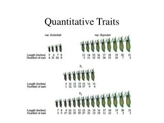
Ch.4 Genetic analysis of quantitative traits. 1. Component of quantitative genetic variation 2. Variance component of a quantitative trait in the populations 3. Heritability ( 유전력 , 유전율 ) 4. QTL analysis. Quantitative traits

E N D
Ch.4 Genetic analysis of quantitative traits 1. Component of quantitative genetic variation 2. Variance component of a quantitative trait in the populations 3. Heritability (유전력, 유전율) 4. QTL analysis
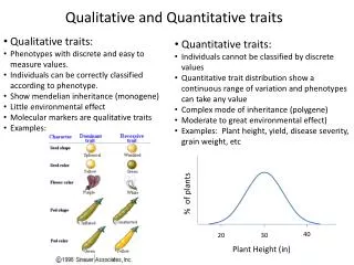
Quantitative traits - described in terms of the degree of expression: metric traits - continuous variation - under polygenic control - influenced by environments - population genetics 1. Component of quantitative genetic variation (1) Types of gene action a. an additive portion : describing the difference between homozygotes at any single locus (Aa = ½(AA + aa) b. a dominance components : arising from interaction of alleles ---> intra-locus interaction (Aa > ½(AA + aa) c. an epistatic part ; associated with interaction of non-alleles ---> inter-locus interaction or epistasis * Application to plant breeding : in choosing parents for crossing and breeding methods to maximize the selection gain
Gene models (Allard) for the expression of a quantitative trait a. Model 1 : additive model b. Model 2 : dominance model c. Model 3 : Epistasis --- complementary model d. Model 4 complex model
2. Variance component of a quantitative trait in the populations • 1) F2 • - Genotypic value • Frequency ¼ ½ ¼ • - Generation mean of F2 = ¼(-da) + ½(ha) + ¼(da) = ½ha • - Variance of F2 = ¼(da-½ha)2 + ½(ha-½ha)2 + ¼(-da-½ha)2 = ½da2 + ¼ha2 • * Many independent loci are involved for the trait ; A-a, B-b, C-c, ... • (Assume that the effects of the genes are cumulative) • da2 + db2 + dc2 + ... = D (Variance for additive effects of genes) • ha2 + hb2 + hc2 + ... = H (Variance for dominant effects of genes) • Then, VF2 = ½ D+ ¼ H + E1 (environmental variance among individuals) Epiatisis, GxE not included 2) VB1, VB2 VB1 : F1 (Aa) x P1 (AA) ---> AA : Aa= 1 : 1 Genotype Freq. Genotypic value Generation mean of B1 AA ½ da ½da+ ½ha Aa ½ ha VB1 = ½ (da-½da-½ha)2 + ½ (ha-½da-½ha)2 = (½da-½ha)2 + E1 Aa AA aa -da ha VB2 : F1 (Aa) x P2 (aa) ---> Aa : aa = 1 : 1 Genotype Freq. Genotypic value Generation mean of B2 Aa ½ ha ½ha - ½da aa ½ -da VB2 = ½ (ha-½ha+½da)2 + ½ (-da-½ha+½da)2 = (½da+½ha)2 + E1 ==> VB1 + VB2 = ½da2 + ½ha2 + 2E1 = ½ D + ½ H + 2E1 +da 0
3) VF3 (Variance of F3 population) Genotype Freq. Genotypic value Mean AA 3/8 da Aa 2/8 ha ¼ ha (=3/8 da + 2/8 ha -3/8 da) aa3/8 -da VF3 = ⅜(da-¼ha)2 + ¼(ha-¼ha)2 + ⅜(-da-¼ha)2 = ¾da2 + 3/16 ha2 + E1 = ¾ D+ 3/16 H+ E1 4) VF3(Variance among F3 lines) (F2) Genotype of F3 lines Freq. Mean of each line Grand mean of lines AA ---> AA ¼ da ¼ha Aa ---> ¼AA+½Aa+¼aa ½ ½ha(=¼da+½ha-¼da) (= ¼da+½(½ha)-¼da) aa---> aa ¼ -da VF3 = ¼(da-¼ha)2 + ½(½ha-¼ha)2 + ¼(-da-¼ha)2 = ½da2 + 1/16 ha2 = ½ D + 1/16 H + E2 (Environm. variation among lines) 5) VF3(Mean of variance of each F3 line) Genotype of lines Freq. Mean of each line Variance within line AA ¼ da 0 ¼AA+½Aa+¼aa ½ ½ha(=¼da+½ha-¼da) ½da2+¼ha2 aa ¼ -da 0 VF3 = ¼(0) + ½ (½da2+¼ha2) + ¼(0) = ¼da2 + ⅛ha2 = ¼ D + ⅛ H + E3 (Mean of environmental variance within line ( ≒ E1)) 6) WF2/F3 (Covcariance between a F2 individual and the F3 line) F2 ind. Value F3 line Value 1/n {∑(x-x)(y-y)} ¼ AA da ¼ AA da ¼ (da-½ha)(da-¼ha) ½ Aa ha ½ (¼AA+½Aa+¼aa) ½ha ½ (ha-½ha)(½ha-¼ha) ¼ aa -da ¼ aa -da ¼ (-da-½ha)(-da-¼ha) Mean ½ha ¼ha +)_______________________ ½ da2 + ⅛ ha2 W F2/F3 = ½ D+ ⅛ H
3. Heritability (유전력, 유전율) Phenotype = Genotype + Environment + GxE Vph= VG + VE + VGxE = VA + VD + VE + VGxE(+ VEpi + Vinteractions) * V: variance, Ph: phenotypic, G: genotypic, E: environmental A: additive, D: dominant, Epi: epistatic Broad sense heritability: the proportion of observed variation in a particular trait that can be attributed to inherited genetic factors in contrast to environmental ones (h2B) h2B = (x 100 %) Narrow sense heritability (h2N) : more useful h2N = *rice 20 vars. 3 repl. IITA, Afr. J. Plant Sci. 5(3): 207-212,
- Heritability for a certain trait is a measure of the response to selection of the trait. The higher the heritability of a trait, the easier it is to modify that trait by selection. If heritability is very high, then phenotypic value is a good estimator of genotypic value. - Although the heritability of a trait depends on how it is measured, in what environment(s) it is measured, and which plant materials are measured. Qualitative traits, such as flower color, often have a value of heritability close to 100. Calculation of Heritability (1) Use of variances in parents, F1, F2: VP , VF1 , VF2 --- h2B VF2 : Variance of F2 population VE : Variance caused by environments -- variation among individuals of the same genotype
(2) Heritability estimation by ANOVA analysis --- h2B n varieties, r replication Ex) barly20 vars. 3 repl(RBD)--- no. of kernels per spike ANOVA df MS F EMS Total 59 530 Variety19 410 ** σE2 + rσg2 Block 2 70 ns σE2 + nσB2 Error 38 50 σE2 σg2 = = 120 h2 = = 0.706 (= 70.6 %) 3
(3) Heritability estimation by variance component method E1 : Variance among individuals of parents E2 : Variance among lines of parents E3 : Mean variance among lines of parents Ex) Oats seed length data collected in an F2 population and F3 lines E1 = 0.3427, E2 =0,0495, E3 =0.3110 Since there are experimental errors in each components across populations calculate an optimum estimates of each component using least square method
i) D ii) For other components, H, E1, E2, E3 iii) Optimum estimate of each components iv) Heritability D = 1.3211 H = 1.0694 E1 = 0.3653 E2 = 0.1015 E3 = 0.3169 In F2 pop. In F3 lines
(4) Use of parent-offspring regression b: regression coefficient rxy: probability which a specific gene of offspring is identical to that of parents h2N= b : in completely heterozygous parents vs offsprings h2N = 2b : in bisexual populations Parent-offspring Regression rxyh2N F1 --> F2 1/2 b F2 --> F3 3/4 2/3 b F3 --> F4 7/8 4/7 b F4 --> F5 15/16 8/15 b F5 --> F6 31/32 16/31 b Ex) In a soybean population (Wiggins, 2012) h2N= 16/31 b = 0.222 (22.2%)
(5) Selection experiment = M’’ – M : response to selection (Rs); selection gain (Gs) ; genetic advance after selection = M’ – M : Selection differential (선발차) = q = selection intensity (out of total) : standard deviation of the trait in the pop. Base population q Freq. M’ M Population after selection value determined by q M Character value M’’
Application of heritability in plant breeding heritability of target traits Prediction of expected gain after selection - across environments - under different experimental designs - using several type of populations + information about the relative costs to determine the optimal selection strategy to make the breeding scheme efficient