Fitting a line to N data points – 1
100 likes | 326 Vues
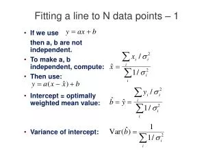
Fitting a line to N data points – 1. If we use then a, b are not independent. To make a, b independent, compute: Then use: Intercept = optimally weighted mean value: Variance of intercept:. Fitting a line to N data points – 2. Slope = optimally weighted mean value:

Fitting a line to N data points – 1
E N D
Presentation Transcript
Fitting a line to N data points – 1 • If we use then a, b are not independent. • To make a, b independent, compute: • Then use: • Intercept = optimally weighted mean value: • Variance of intercept:
Fitting a line to N data points – 2 • Slope = optimally weighted mean value: • Optimal weights: • Hence get optimal slope and its variance:
Linear regression • If fitting a straight line, minimize: • To minimize, set derivatives to zero: • Note that these are a pair of simultaneous linear equations -- the “normal equations”.
The Normal Equations • Solve as simultaneous linear equations in matrix form – the “normal equations”: • In vector-matrix notation: • Solve using standard matrix-inversion methods (see Press et al for implementation). • Note that the matrix M is diagonal if: • In this case we have chosen an orthogonal basis.
General linear regression • Suppose you wish to fit your data points yi with the sum of several scaled functions of the xi: • Example: fitting a polynomial: • Goodness of fit to data xi, yi, i: • where: • To minimise 2, then for each k we have an equation:
Normal equations • Normal equations are constructed as before: • Or in matrix form:
Uncertainties of the answers • We want to know the uncertainties of the best-fit values of the parameters aj . • For a one-parameter fit we’ve seen that: • By analogy, for a multi-parameter fit the covariance of any pair of parameters is: • Hence get local quadratic approximation to 2 surface using Hessian matrix H:
The Hessian matrix • Defined as • It’s the same matrix M we derived from the normal equations! • Example: y = ax + b.
b a b a Principal axes of 2 ellipsoid • The eigenvectors of H define the principal axes of the 2 ellipsoid. • H is diagonalised by replacing the coordinates xi with: • This gives • And so orthogonalises the parameters.
Principal axes for general linear models • In the general linear case where we fit K functions Pk with scale factors ak: • The Hessian matrix has elements: • Normal equations are • This gives K-dimensional ellipsoidal surfaces of constant 2 whose principal axes are eigenvectors of the Hessian matrix H. • Use standard matrix methods to find linear combinations of xi, yi that diagonalise H.