Chapter 8 – Expenditure Programs for the Poor

1. Chapter 8 – Expenditure Programs for the Poor Public Economics

2. Quick Look at Welfare Spending • “Welfare” in the United States is a patchwork of dozens of different programs. • All welfare programs are means-tested – only individuals with sufficiently low income are eligible. • Programs often have other requirements related to family structure and assets.

3. Quick Look at Welfare Spending • Spending on welfare programs, as a fraction of GDP, has more than double in the past 30 years. • The role of direct cash assistance has diminished, however. Subsidized health care has grown enormously.

4. Table 8.1

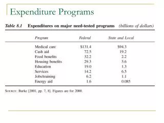
5. Quick Look at Welfare Spending • Table 8.1 shows that welfare spending is a shared expense between the federal and state/local governments. • Subsidized medical care (mainly Medicaid) exceeded $215 billion in 2000. • Cash assistance (including the Earned Income Tax Credit) exceeded $91 billion in 2000.

6. TANF • 1935-1996: AFDC • Aid to Families with Dependent Children • 1996-present: TANF • Temporary Assistance for Needy Families • Programs are largely targeted toward single parent households with children under 18.

7. AFDC Open-ended entitlement – anyone who qualifies gets AFDC. No time limits – could be on program indefinitely No work requirements Cost sharing by federal and state governments – open ended costs. State determines benefit levels subject to broad federal guidelines High tax rates on earned income TANF No “entitlement” – limited funding. Time limited for at most 5 years Work requirements Block grant to states – costs to federal government are not open ended. States have even more control of the design of the program States have option to lower tax rates on earned income AFDC/TANF differences

8. TANF • Benefit reduction rates (also known as tax rates) vary from 33% to 100%. • 100% tax rate means that if a welfare recipient earns $1 in the labor market, her welfare benefit is reduced by exactly $1.

9. TANF • Welfare grant levels vary tremendously • More than cost-of-living differences alone could explain • For a 3-person family with no other sources of income, grant was: • $801 for the family each month in Minnesota • $164 for the family each month in Alabama

10. Income Maintenance and Work Incentives • Analyzing welfare programs is simply utility maximization subject to a budget constraint. • The government’s welfare program design changes the budget constraint, and the economic agent then maximizes utility.

11. Income Maintenance and Work Incentives • In the simplest possible case, a state’s welfare program can be characterized by two variables: • G – the basic grant the individual receives when not working. • t – the rate at which the grant is taken away when the recipient earns income; the tax rate.

12. Income Maintenance and Work Incentives • For example, suppose a state gives a grant of $300, but benefits are reduced by 25 cents for each dollar earned. • G=300 and t=0.25 • If the individual earns $500, her welfare benefit is reduced from $300 to ($300-0.25*500), or $175. • Eventually, the person will earn too much money to qualify for any welfare benefit.

13. Income Maintenance and Work Incentives • Algebraically, the actual benefit received (B) is related to the tax rate (t), welfare grant (G), and actual earnings (E).

14. Income Maintenance and Work Incentives • When benefits fall to zero (B=0), the person is no longer eligible for welfare. This implies: • When a welfare system only has two features, G and t, the above equation tells the earnings level where welfare eligibility ends.

15. Income Maintenance and Work Incentives • This formula is called the “break-even” level. • It highlights the fundamental tradeoff in welfare program design: • Lower tax rates, t, provide better work incentives for welfare recipients, but make more people eligible. • For example, with G=300 and t=0.25, the income eligibility limit is $1200. • With a much higher tax rate of 100%, the income eligibility limit is $300. • Fewer people qualify with the 100% tax rate, but such a high tax could discourage work among welfare recipients.

16. Analysis of work incentives • Typical utility maximization problem includes a utility function (U), prices of goods (p), and income (I). • The key change in an analysis of labor supply and welfare programs is that rather than being “endowed” with income, the person is endowed with time, T. • This is known as the time endowment – which can be used for either labor or leisure.

17. Analysis of work incentives • The utility function consists of two goods, leisure and “all other consumption goods” (which will simply be measured as income in the examples below). • U=u(L,C) or equivalently U=u(L,I) where • L=Leisure • C=Consumption goods • I=income

18. Analysis of work incentives • This utility function shows that leisure is a “good” – all else equal, people prefer more to less. • The reason why people work is to buy consumption goods. • If we denote H=hours of work, then: • L+H=T • The amount of leisure and hours of work equals the time endowment.

19. Figure 8.1

20. Analysis of work incentives • In Figure 8.1, the x-axis therefore simultaneously represents leisure (moving away from the origin), and hours of work (moving toward the origin). • Oa represents hours of leisure, and aT represents hours of work. • The y-axis represents consumption goods or income (they are interchangeable).

21. Analysis of work incentives • In Figure 8.1, if the person does not work at all, then L=T (H=0). Smith earns no money, and therefore has zero income (consumption goods). • Thus, one point on her budget constraint is {T,0}

22. Analysis of work incentives • If she gives up one hour of leisure, she works one hours and earns a wage rate of w. • Thus, another point on her budget constraint is {T-1,w}, which is labeled as point b. • If she gives up two hours of leisure, she works two hours and earns a wage rate of 2w. • Thus, another point on her budget constraint is {T-2,2w}, which is labeled as point c.

23. Analysis of work incentives • The most leisure she could give up is T hours (her time endowment), which leads to y-intercept on her budget constraint: {0,Tw}. • This exercise traces out all the leisure/income combinations along the line TD. • The price of an additional hour of leisure is its opportunity cost – the income forgone by not working that hour – which is the wage rate, w.

24. Analysis of work incentives • Given this budget constraint, the person maximizes utility by choosing the indifference curve tangent to the budget constraint. • This is illustrated in Figure 8.2. • The amount of leisure consumed is OF. • The amount of income is OG.

25. Figure 8.2

26. Numerical example • Assume that Smith has the following preferences over leisure and consumption goods: • Further, assume that the price of leisure is $5, price of consumption goods is $2, and the time endowment is 100 hours.

27. Numerical example • The “full” budget constraint is therefore: • In general, the demand curve for good X in a Cobb-Douglas utility function of the form: is

28. Numerical example • This translates easily into leisure demand: • She therefore consumes 25 hours of leisure (provides 75 hours of work), earns $375 (=75x$5), and purchases 187.5 units of consumption goods (=$375/2).

29. Introducing the welfare system into the analysis • In the previous figures, the person would literally starve if she did not work at all. • The welfare system provides additional income for those with low earnings (low hours of work). • Figure 8.3 illustrates the budget constraint with grant of $100 and a tax rate of 25%.

30. Figure 8.3

31. Introducing the welfare system into the analysis • In Figure 8.3, the budget constraint has changed with the introduction of the welfare system. • If the person does not work, she now collects $G from the welfare system. • Thus, point Q represents the leisure/income combination {T,G}.

32. Introducing the welfare system into the analysis • As she begins to work, she still receives w from her employer, but her grant is reduced by tw, or 0.25w. • Her income therefore increases by 0.75w, not w, from an additional hour of work. • The (absolute value) of the slope is flatter than before.

33. Introducing the welfare system into the analysis • Where does she lose welfare benefits? Answer: when her benefits fall to zero, which occurs at the “breakeven level.” • The earnings where welfare eligibility is lost is equal to:

34. Introducing the welfare system into the analysis • The hours of work where welfare eligibility is therefore: • It follows that the leisure where welfare eligibility ends is:

35. Introducing the welfare system into the analysis • In Figure 8.3, this expression for leisure corresponds to OV. • After earning this amount, Smith no longer collects welfare benefits, and gets to keep the entirely hourly wage. • Thus, the new budget constraint is given by the kinked line QSD.

36. Introducing the welfare system into the analysis • How will Smith react to the new budget constraint QSD rather than TD? • It will depend on her indifference curves. • Given the indifference curves in Figure 8.4, Smith reduces her hours of work from FT to KT. Her leisure increases from OF to OK.

37. Figure 8.4

38. Introducing the welfare system into the analysis • Note that Smith is clearly better off in Figure 8.4 after the welfare system is introduced – her utility is higher than before.

39. Introducing the welfare system into the analysis • In the previous case, we assumed the tax rate was t=25%. • The next case considers a higher tax rate, t=100%.

40. Introducing the welfare system into the analysis • Note that 100% tax rates are not unheard of in the welfare system. • Nine states and the District of Columbia impose this tax rate. • Assume that G=$338 per month.

41. Introducing the welfare system into the analysis • Now, when a welfare recipient works another hours and earns w, her welfare benefit is reduced by exactly w. • Her net wage is therefore $0! • She moves from {T,$338} to {T-1,$338} • This is illustrated as P1 in Figure 8.5. • Regardless of her preferences, she would never choose point P1 because it violates the non-satiation assumption.

42. Figure 8.5

43. Introducing the welfare system into the analysis • The breakeven level of earnings is G/t=($338/1.0)=$338. • After Smith earns $338, her welfare benefit has fallen to zero, and she then keeps all of her additional earnings. • The absolute value of the slope of the budget constraint becomes w. • The budget constraint is therefore PRD.

44. Introducing the welfare system into the analysis • Given the 100% tax rate, and Smith’s indifference curves in Figure 8.6, she rationally chooses to leave the labor force, and consume {T,338}.

45. Figure 8.6

46. Introducing the welfare system into the analysis • It is never rational in Figure 8.6 to work between 0 and PR hours. • This special case does not explicitly depend on a person’s indifference curves, because the tax rate is 100%.

47. Introducing the welfare system into the analysis • It is not true, however, that all people leave the labor force when the tax rate on welfare benefits is 100%. • Figure 8.7 illustrates a person with a high level of work effort, who attains higher utility at E2 than at P.

48. Figure 8.7

49. Introducing the welfare system into the analysis • This person’s indifference curve is everyone above the welfare part of the budget constraint. • If the welfare grant, G, increased sufficiently, at some point this person would respond by leaving the labor force (assuming t=100%). • But the current grant level in Figure 8.7 does not induce this person to leave.

50. Introducing the welfare system into the analysis • Why impose such high tax rates if these tax rates create work disincentives? • Holding the grant constant, lowering the tax rate increases welfare eligibility. For example, lowering t in the previous figure (Figure 8.7) would eventually induce this person to enter welfare.