Download
1 / 21
220 likes | 448 Vues
z-Scores. The z-score is often called the standardized value. It denotes the number of standard deviations a data value x i is from the mean. Excel’s STANDARDIZE function can be used to compute the z-score. z-Scores. An observation’s z-score is a measure of the relative

E N D
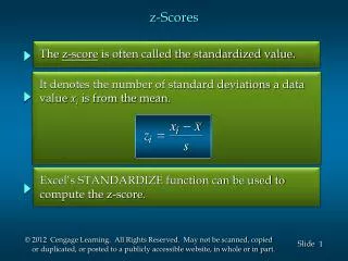
z-Scores The z-score is often called the standardized value. It denotes the number of standard deviations a data value xi is from the mean. Excel’s STANDARDIZE function can be used to compute the z-score.
z-Scores • An observation’s z-score is a measure of the relative location of the observation in a data set. • A data value less than the sample mean will have a • z-score less than zero. • A data value greater than the sample mean will have • a z-score greater than zero. • A data value equal to the sample mean will have a • z-score of zero.
Chebyshev’s Theorem At least (1 - 1/z2) of the items in any data set will be within z standard deviations of the mean, where z is any value greater than 1. Chebyshev’s theorem requires z > 1, but z need not be an integer.
Chebyshev’s Theorem At least of the data values must be within of the mean. 75% z = 2 standard deviations At least of the data values must be within of the mean. 89% z = 3 standard deviations At least of the data values must be within of the mean. 94% z = 4 standard deviations
Let z = 1.5 with = 490.80 and s = 54.74 - z(s) = 490.80 - 1.5(54.74) = 409 + z(s) = 490.80 + 1.5(54.74) = 573 Chebyshev’s Theorem • Example: Apartment Rents At least (1 - 1/(1.5)2) = 1 - 0.44 = 0.56 or 56% of the rent values must be between and (Actually, 86% of the rent values are between 409 and 573.)
99.72% 95.44% 68.26% Empirical Rule x m m + 3s m – 3s m – 1s m + 1s m – 2s m + 2s
Covariance The covariance is a measure of the linear association between two variables. Positive values indicate a positive relationship. Negative values indicate a negative relationship.
Covariance The covariance is computed as follows: for samples for populations
Correlation Coefficient Correlation is a measure of linear association and not necessarily causation. Just because two variables are highly correlated, it does not mean that one variable is the cause of the other.
Correlation Coefficient The correlation coefficient is computed as follows: for samples for populations
Correlation Coefficient The coefficient can take on values between -1 and +1. Values near -1 indicate a strong negative linear relationship. Values near +1 indicate a strong positive linear relationship. The closer the correlation is to zero, the weaker the relationship.
Covariance and Correlation Coefficient • Example: Golfing Study A golfer is interested in investigating the relationship, if any, between driving distance and 18-hole score. Average Driving Distance (yds.) Average 18-Hole Score 69 71 70 70 71 69 277.6 259.5 269.1 267.0 255.6 272.9
Covariance and Correlation Coefficient • Example: Golfing Study x y 69 71 70 70 71 69 -1.0 1.0 0 0 1.0 -1.0 277.6 259.5 269.1 267.0 255.6 272.9 10.65 -7.45 2.15 0.05 -11.35 5.95 -10.65 -7.45 0 0 -11.35 -5.95 Average Total 267.0 70.0 -35.40 Std. Dev. 8.2192 .8944
Covariance and Correlation Coefficient • Example: Golfing Study • Sample Covariance • Sample Correlation Coefficient
Grouped Data • The weighted mean computation can be used to • obtain approximations of the mean, variance, and • standard deviation for the grouped data. • To compute the weighted mean, we treat the • midpoint of each class as though it were the mean • of all items in the class. • We compute a weighted mean of the class midpoints • using the class frequencies as weights. • Similarly, in computing the variance and standard • deviation, the class frequencies are used as weights.
Mean for Grouped Data • Sample Data • Population Data where: fi = frequency of class i Mi = midpoint of class i
Sample Mean for Grouped Data • Example: Apartment Rents The previously presented sample of apartment rents is shown here as grouped data in the form of a frequency distribution.
Sample Mean for Grouped Data • Example: Apartment Rents This approximation differs by $2.41 from the actual sample mean of $490.80.
Variance for Grouped Data • For sample data • For population data
continued Sample Variance for Grouped Data • Example: Apartment Rents
Sample Variance for Grouped Data • Example: Apartment Rents • Sample Variance s2 = 208,234.29/(70 – 1) = 3,017.89 • Sample Standard Deviation This approximation differs by only $.20 from the actual standard deviation of $54.74.