Download
1 / 37
370 likes | 390 Vues
OMI UV spectral irradiance: comparison with ground based measurements in an urban environment. Stelios Kazadzis A. Bais, A. Arola OMI science team meeting Helsinki, June 2008 Finnish Meteorological Institute Laboratory of Atmospheric Physics, Thessaloniki, Greece. Outline.

E N D
OMI UV spectral irradiance: comparison with ground based measurements in an urban environment Stelios Kazadzis A. Bais, A. Arola OMI science team meeting Helsinki, June 2008 Finnish Meteorological Institute Laboratory of Atmospheric Physics, Thessaloniki, Greece
Outline • OMI – ground based UV spectral irradiance comparison – statistics • Aerosol absorption – post correction approaches • Campaign: Spacial and temporal UV variability within an OMI grid Stelios Kazadzis, OMI science team meeting Helsinki, June 2008
OMI – GB UV comparison – statistics • The problem - absorbing aerosols Current OMI UV algorithm does not account for absorbing aerosols (e.g. organic carbon, smoke, dust ) Tokyo: +32% Tanskannen et al., JGR 2007 Stelios Kazadzis, OMI science team meeting Helsinki, June 2008
OMI – GB UV comparison – statistics Thessaloniki Area • High aerosol load- Aerosol transportSahara dust intrusions Biomass burning from NE- Very high PM10 conc. Sahara - Dream model Fire hot spots - summer Stelios Kazadzis, OMI science team meeting Helsinki, June 2008
OMI – GB UV comparison – statistics Instrumentation - comparison Thessaloniki September 2004-December 2007 Brewer instrument(spectral-calibrated, wavelength shift corrected)UV irradiance at 305, 324, 380 nm and CIETotal column ozonespectral AOD at UV wavelengths CIMELAOD (340nm) , SSA(440nm), ..NILU-UV 305nm, 324nm, 340nm, 380nmCloud – cloudless case separationPyranometer, observations, sky camera pixDaily OMI overpass time (mean over ±15 minutes) Rooftop of the School of Natural Sciences Stelios Kazadzis, OMI science team meeting Helsinki, June 2008
OMI – GB UV comparison – statistics Results 305nm OMI +30%324nm OMI +17% Stelios Kazadzis, OMI science team meeting Helsinki, June 2008
OMI – GB UV comparison – statistics Results 380nm OMI +11%CIED OMI +20% Stelios Kazadzis, OMI science team meeting Helsinki, June 2008
OMI – GB UV comparison – statistics Results - statistics Stelios Kazadzis, OMI science team meeting Helsinki, June 2008
OMI – GB UV comparison – statistics Results - statistics Stelios Kazadzis, OMI science team meeting Helsinki, June 2008
Arola et al., JGR 2005 Krotkov et al., OE 2004 Post correction methods Post correction methods - TOMS experience Cloudless cases: Ta(λ) = AOD(λ) * [1 - SSA(λ)] Stelios Kazadzis, OMI science team meeting Helsinki, June 2008
Post correction methods UV attenuation – Thessaloniki, cloudless cases Stelios Kazadzis, OMI science team meeting Helsinki, June 2008
Post correction methods Post correction : method 1 Ta (λ) = AOD(λ) * [1 - SSA(440nm)] Aerosol absorption CF(λ) = 1.1 + 1.5 * Ta(λ) • no sza dependence • SSA @ UV ? • need of GB data Stelios Kazadzis, OMI science team meeting Helsinki, June 2008
Post correction methods Post correction: method 2 Tas =Ta / cos(sza) Aerosol absorption CF(λ) = 1.07 + 1.8 * Tas(λ) • SSA @ UV ? • need of GB data Stelios Kazadzis, OMI science team meeting Helsinki, June 2008
Post correction methods Post correction: use of RT model Abs + scat scat S1: AOD and SSA synchronous measurementsS2: AOD and SSA@440 = constS3: AOD= const and SSA@340 = const Stelios Kazadzis, OMI science team meeting Helsinki, June 2008
Post correction methods Overview of post corrections 6th Approach: CF(λ) = 1 + 3 * Ta(λ) Table with all the results of the 6 approaches: Stelios Kazadzis, OMI science team meeting Helsinki, June 2008
Post correction methods Overview of post corrections 6th Approach: CF = 1 + 3 * Ta(λ) Table with all the results of the 6 approaches: Stelios Kazadzis, OMI science team meeting Helsinki, June 2008
Post correction methods Overview of post corrections 6th Approach: CF = 1 + 3 * Ta(λ) Table with all the results of the 6 approaches: Stelios Kazadzis, OMI science team meeting Helsinki, June 2008
Post correction methods Overview of post corrections 6th Approach: CF = 1 + 3 * Ta(λ) Table with all the results of the 6 approaches: Stelios Kazadzis, OMI science team meeting Helsinki, June 2008
Post correction methods Correction results 305nm +11% 324nm +2% 380nm +0% Stelios Kazadzis, OMI science team meeting Helsinki, June 2008
Post correction methods Effects of sza, AOD, SSA, ozone, time on ratios Stelios Kazadzis, OMI science team meeting Helsinki, June 2008
Spatial and temporal UV variability within an OMI grid Campaign: 1 to 30 October, 2007 • 3 sitesEach:NILU UV at 305, 324, 380nmCIMEL (AOD, SSA, ..) Pyranometer, sky cameraMain site+ Brewers Spectral UV, ozoneCCD (spectral AOD) 2 Lidars (City – Rural) Stelios Kazadzis, OMI science team meeting Helsinki, June 2008
Spatial and temporal UV variability within an OMI grid UV Measurements at the three sites Stelios Kazadzis, OMI science team meeting Helsinki, June 2008
Spatial and temporal UV variability within an OMI grid AOD variability in an OMI grid Stelios Kazadzis, OMI science team meeting Helsinki, June 2008
Spatial and temporal UV variability within an OMI grid UV differences in an OMI grid +20% -20% Stelios Kazadzis, OMI science team meeting Helsinki, June 2008
Spatial and temporal UV variability within an OMI grid Spatial UV variability at 3 stations (2 * sigma / mean)*100 Stelios Kazadzis, OMI science team meeting Helsinki, June 2008
Spatial and temporal UV variability within an OMI grid Temporal UV variability (2 * sigma / mean)*100 Stelios Kazadzis, OMI science team meeting Helsinki, June 2008
Conclusions • 3.5 years of OMI and ground based at Thessaloniki, Greece: measurement comparisonshowed an OMI overestimation of UV irradiances. • Cloudless cases: Main reason is the aerosol absorption. Higher deviations at lower wavelengths • Possible methods to correct this effect: AOD and SSA measurements or/and an aerosol absorption climatology needed in a global scale • SSA in the UV: while mean SSA at 440 nm is 0.90 (Thessaloniki) an SSA of 0.82 is needed for eliminating GB and OMI UV differences at 305nm. SSA at UV-B wavelengths needs further investigation. • Simple public information (e.g. UVINDEX) retrieved from OMI at such populated-urban areas are affected from this bias. +20% on cloudless day. • Aerosol variation within an OMI satellite pixel can cause UV differences equal to a percentage (~18%) that 90% of cloudless comparison cases lie within. Statistical analysis limitations ? • Spatial and temporal UV variability has to be taken into account when comparing GB and satellite UV, especially at city areas. • Comparison under cloudy conditions requires more investigation as absolute differences are large and spatial and temporal UV variability plays a very important role on single station – satellite, comparison. Stelios Kazadzis, OMI science team meeting Helsinki, June 2008
Thank youCampaign acknowledgments:D. Balis, N. Kouremeti, V. Amiridis, M. Zebila,E. Giannakaki, J. Herman, AERONET Stelios Kazadzis, OMI science team meeting Helsinki, June 2008
Spatial and temporal UV variability within an OMI grid OMI – GB normalized biases 3 stations Stelios Kazadzis, OMI science team meeting Helsinki, June 2008
Back up air masses 4 day back traj Stelios Kazadzis, OMI science team meeting Helsinki, June 2008
Back up – Lidar 2 days Stelios Kazadzis, OMI science team meeting Helsinki, June 2008
Back up TOMS and UVA correction Stelios Kazadzis, OMI science team meeting Helsinki, June 2008
Back up Brewer –MODIS (2000-2007) Stelios Kazadzis, OMI science team meeting Helsinki, June 2008
Back up SSA Thessaloniki (1998-2005) Stelios Kazadzis, OMI science team meeting Helsinki, June 2008
Back up SSA scout Stelios Kazadzis, OMI science team meeting Helsinki, June 2008
Spatial and temporal UV variability within an OMI grid • Spectral measurements of direct and global UV irradiance at the surface were made with two Brewer spectroradiometers. In addition, global (diffuse plus direct) UV irradiance and photosynthetically active radiation (PAR) were measured, on a minute basis, at each of the three sites with three NILU-UV multi-channel radiometers. • In-situ measurements of aerosol vertical profiles were derived from two Lidar systems operating at (AUTH) and the site of Epanomi. • Total ozone column was derived from the Brewers and cloud observations and sky images at the AUTH site. Cloud observations were performed at all sites at a half hour basis. • Sun and sky radiance measurements were conducted with three CIMEL automatic sun tracking photometers, each installed at one of the three sites. These data were used to derive aerosol optical properties such as the aerosol optical depth (AOD), the Angstrom exponent a (AEa) and the single scattering albedo (SSA). Stelios Kazadzis, OMI science team meeting Helsinki, June 2008