Spatial point patterns and Geostatistics an introduction
440 likes | 644 Vues
Spatial point patterns and Geostatistics an introduction. Marian Scott Sept 2006. Outline. Spatial point processes Geostatistics The variogram Spatial interpolation and prediction Sampling plans How to do it in R. Spatial point processes.

Spatial point patterns and Geostatistics an introduction
E N D
Presentation Transcript
Spatial point patterns and Geostatisticsan introduction Marian Scott Sept 2006
Outline • Spatial point processes • Geostatistics • The variogram • Spatial interpolation and prediction • Sampling plans • How to do it in R
Spatial point processes • ‘A Spatial point process is a set of locations, irregularly distributed within a designated region and presumed to have been generated by some form of stochastic mechanism’ - Diggle (2003). • A realisation from a spatial point process is termed a spatial point pattern – a countable collection of points {xi}. • When we speak about an event, we mean a single observation xifrom the process. • We denote by N(A), the random variable representing the number of events in the region A. By a point, we simply mean any other arbitrary location.
What is the question? It is natural to ask the following question: • Does each point pattern differ from a random spatial pattern or complete spatial randomness? • what do we mean by complete spatial randomness?.
Complete Spatial Randomness (CSR) Given any spatial region A, CSR asserts that (i) conditional on N(A), the events in A are uniformly distributed over A. (ii) the random variable N(A) follows a Poisson distribution with mean |A|. In (ii) above, is termed the intensity, or the expected number of events per unit of area. A process satisfying (i) and (ii) is called a Spatial Poisson process (with intensity ).
Stationarity and isotropy • Space is like time (in a simple sense) in that our spatial processes should be stationary, but what about isotropy? • Isotropy is: A process is said to be isotropic if the joint distribution of N(A1), . . . ,N(Ak) is invariant to rotations. So in simple terms has to do with directions • Note: The spatial Poisson process is both stationary and isotropic.
Mean and variance equivalents • Called the first order and second order intensity functions • They are the limiting behaviour of the expected value of N(A1) and covariance of N(A1), N(A2)
1st and 2nd order intensity functions • for stationary, isotropic processes: (x) = N(A)/ |A|. = • But 2(x,y) not easy to describe in words, but easier to consider the K-function K(t)=1/ E{N0(t)}, where N0(t) is the number of events within a distance t of an arbitrary event.
Why is the K-function useful? • K(t) =1/ E(number of events within a distance t of an arbitrary event) • This suggests that for clustered patterns, K(t) will be relatively large for small values of t, since events are likely to be surrounded by further members of the same cluster. • While for regularly spaced patterns, small values of t will give relatively small values of K(t) - here there is likely to be more empty space around events.
The K-function can be used to assess CSR • For the case of a Poisson process, Kcsr(t) = t2. • For the case of clustered patterns, we would expect for short distances t that K(t) > t2. • For regular patterns, we would expect that for short distances t that K(t) < t2.
Estimating the K-function • K(t) =1/E(number of events within a distance t of an arbitrary event) • First we need to estimate - the obvious estimator is hat= n/|A| • we can estimate K(t) as an average over all points of the pattern, so using hat we can then estimate K(t) and plot this against the theoretical function for CSR (should be a straight line if CSR reasonable)
Other approaches • Nearest neighbour methods - G-function The empirical distribution function of event-to-event nearest neighbours distances, G(·). • Nearest neighbour methods - F-function The empirical distribution function of point-to-event nearest neighbour distances, F(·) • Tests for CSR For a Poisson process (ie CSR) then the theoretical distribution functions G(s) = F(s) = 1 - exp(-s2)
Further models for Spatial point processes • Poisson cluster process • Inhomogeneous Poisson process • Cox process • Inhibition process
The problem of geostatistics Given observations at n sites Z(u1),…, Z(un) • How best to draw a map? • What is our estimate of Z(u0) where u0 is location of an unobserved site?
Spatial trend- the mean function By definition, a trend is a systematic change in the mean value of the attribute over the area of interest. It is generally recognized that trend is a regional property. Although the trend is usually assumed to be smooth, it may change abruptly in response to sudden changes in environmental forcing variables (e.g., changes in bedrock geology).
The autocovariance function The autocorrelation function
The semi-variogram Variance and covariance as a function of distance separating the locations
Isotropy and stationarity • A spatial random process is said to be isotropic if its properties do not depend on direction. C(t) does not depend on direction • Stationarity means there is no spatial trend, no spatial periodicity, and the spatial covariance is the same at all locations
Isotropy and Stationarity • An isotropic process is one whose properties (in particular the variogram) do not vary with direction • A stationary process is one whose properties do not vary with space • See Richard’s definition of stationarity in time series.
Steps in a geostatistical analysis • Exploration • Estimating the variogram • Spatial interpolation and prediction
Estimating the variogram for i,j=1,..n,
What are the nugget,range and sill? • The nugget is the limiting value of the semivariance as the distance approaches zero. The nugget captures spatial variability at very small spatial scales (those less than the separation between observations) and also measurement error. The sill is the horizontal asymptote of the variogram, if it exists, and represents the overall variance of the random process. The range is the lag value at which the semi-variance value reaches the sill.
Fit a variogram model Rather than look at the empirical variogram we can fit a model. Common examples are a spherical and an exponential variogram
Variogram models The nugget for random data The spherical
Spatial interpolation and prediction • Regression modelling (surface fitting) using generalised least squares • Inverse distance weighted interpolation • kriging
Interpolation at unsampled location u0 The main difference between the different methods is the estimation of the weights
137Cs deposition maps in SW Scotland prepared by different European teams (ECCOMAGS, 2002)
Geostatistical model • The sample data,zi , are considered as realizations of a spatial random process,Z(u), with the sample points,ui , located in a two-dimensional spatial domain. That is,ui is a set of vectors. The process Z(u) is often assumed to be Gaussian.
Geostatistical model • where represents the non-stochastic spatial component of the random process or trend; Sr is the stochastic part of the process. The variance of Z(u) is defined by the variance of the stochastic part of the process namely .2 .
Kriging 1 Ordinary kriging First, the trend is estimated and subtracted from the observations. After the trend is estimated, the observed values can be de-trended by subtracting the estimated trend. Then, the variogram value and the distance between the locations are calculated for each pair of de-trended observations A model for the variogram is then fit and used to generate the weights for the weighted average process
Kriging 2 Other methods of kriging There are a number of other kriging methods, such as block kriging, indicator kriging and co-kriging Some interesting issues concern the uncertainty, we can use the kriging procedure to produce and uncertainty map and recent work has been to develop approaches to incorporate the uncertainty in the variogram model.
Other uses of the variogram The variogram provides information about the spatial correlation between locations. If goal is to produce a map, need to detect small-scale fluctuations in the quantity of interest. Prediction of the values at individual locations is most precise when those locations are highly correlated with observed locations. This can be achieved by ensuring that no place on the map is too far from an observed location One design to achieve this is a systematic sample with a grid spacing less than the range of the variogram.
Other uses of the variogram If the sampling goal is to estimate the average over the entire study area, the opposite strategy is more appropriate. Correlated observations provide redundant statistical information, so it would be appropriate to spread out points so that no distance between a pair of points is smaller than the variogram range.
Kriging in R There are routines to do kriging in the R libraries:- geoR fields gstat sgeostat spatstat spatdat