Executive Functions and Control of Processing
Executive Functions and Control of Processing. PDP Class March 2, 2011. The Stroop Task(s): Read Word. RED GREEN BLUE GREEN BLUE RED BLUE RED GREEN BLUE GREEN. The Stroop Task: Name Ink Color. BLUE RED BLUE RED GREEN BLUE GREEN RED GREEN BLUE GREEN.

Executive Functions and Control of Processing
E N D
Presentation Transcript
Executive Functions and Control of Processing PDP Class March 2, 2011
The Stroop Task(s):Read Word RED GREEN BLUE GREEN BLUE RED BLUE RED GREEN BLUE GREEN
The Stroop Task:Name Ink Color BLUE RED BLUE RED GREEN BLUE GREEN RED GREEN BLUE GREEN
Reaction Time Data from a Stroop Experiment Color naming Word reading
Alternative Views of the Role of Control and Attention • Two kinds of processing: Controlled processing and automatic processing • One slow and effortful, the other fast and effort-free • One kind of processing, varying in ‘pathway strength’ • When strength is low, control is necessary to allow the pathway to control behavior • When strength is high, control is necessary to prevent the pathway from controlling behavior
A Model of Control of Automatic Processing in the Stroop Task (Cohen, Dunbar, and McClelland, 1990) • Model employs a feed-forward, non-linear activation process so that color and word input can activate response units. • neti(t) = l Saj(t)wij(t) + (1-l)neti(t-1) • ai(t) = logistic(neti(t)) • Activation builds up over time (rate controlled by l). • Speed and automaticity of processing depends on strengths of connections. • Connections are stronger for word than for color, so that the word tends to dominate activation of output units. • Activation coming from ‘task demand’ units provides an additional source of input that can regulate the ‘strength’ of each pathway. • This instantiates the ‘Biased Processing’ model of control of behavior and attention. • The effect is graded so that strong pathways tend to influence performance even when it would be best if their influence could be prevented.
The Cohen et al Stroop model (fully ‘feed-forward’)
How Task Biases Processing in the Stroop Model • Input from task demand units sets the baseline net input for the hidden units. • Stimulus effects add or subtract from the baseline. • The same size stimulus effect has a bigger effect on activation of units when the baseline is near the middle of the range than when it is down near the bottom. • This allows task to amplify task-relevant input to the output units, relative to task-irrelevant inputs.
How the model accounts for key features of the data • Left panel below shows how asymptotic activation of response units tends to be more affected by inhibition (as in conflict trials) than excitation (as in congruent trials). • Right panel shows how this translates into more slowing of performance (interference) on conflict trials than speeding of performance (facilitation) on congruent trials. < response threshold Time to reachthreshold for different conditions Net input and activationat asymptote Build up of activation over time
Effect of practice using color words as names for arbitrary shapes on naming the shape and the shape’s color
AX-CPT: Experimentaland SimulationResults • First-episode schizophrenics show a deficit only at a long delay, while multi-episode schizophrenics show a deficit at both the short and long delay. • Must we postulate two different deficits? • Braver et al suggest maybe not, since different degrees of gain reduction can account for each of the two patterns of effects. • The performance measure represents the degree to which responding at the time of probe presentation (X) is modulated by prior context (A vs. non-A).
Take-Home Message from the work of Cohen et al. • In these models, deficits that look like failures to inhibit pre-potent responses and deficits that look like failures of working memory both arise as a consequence of reduced activation of units responsible for maintained activation of task or context information in a form that allows it to exert control over processing. • Thus, the authors suggest, the crucial role of the PFC is to provide the mechanism that maintains this sort of information. • The exertion of control requires connections from PFC so that specific content maintained in PFC exerts control on appropriate specific neurons elsewhere.
Evidence for a hierarchy of control • Velanova et al (J. Neurosci, 2003) contrasted low vs. high control (well-studied vs. once-studied) retrieval conditions. • Upper panel shows left Lateral PFC region showing greater transient activity in the high control condition. • Lower panel shows right fronto-polar region showing sustained activity in the high control condition (left) but not the low-control condition (right). • From this they argue for a hierarchy of control, with fronto-polar cortex maintaining overall task set and Lateral PFC playing a transient role in controlling memory search on a trial-by trial basis. • Ideas about the role of particular PFC regions have continued to grow more and more complex…
But what’s controlling the controller (that’s controlling the controller)? • Is there an infinite regress problem in cognitive control? • One way to break out of it is with a recurrent network. • Learned connection weights in the network can allow an input to set up a state that persists until another input comes in that sets the network in a different state. • A model of performance in a working memory task is shown on the next slide.
Working Memory TaskStudied by Pelegrino Et Aland Modeled by Moody Et al
Moody et al’s Network Network is trained to ‘load’ x-y value when presentedwith ‘gate’, continue to output x and y while viewingtest distractors, then produce a ‘match’ response when thetest stimulus matches the sample.
A storage cell: - firing starts and ends with match - activation is unaffected by distractors
How do we usually maintain information? • While Moody et al treat the maintenance of information as a function solely of pre-frontal cortex, others (esp. Fuster) have argued that maintenance is generally a function of a multi-regional maintained activation state in which the PFC plays a role but so does sustained activity in posterior cortex. • This of course is more consistent with a PDP approach.
Control as an Emergent Process: Botvinick and Plaut (2004) Model of Action, Action Slips, and Action Disorganization Syndrome • Model is a simple recurrent network trained to make coffee or tea (with cream and/or sugar). • Network is trained on valid task sequences. • Input at the start of a sequence can specify the task (coffee/tea; cream/sugar), but goes away; network must maintain this. • At test, it is given a starting input, then its inputs are updated given its actions. • Slips and A.D.S. are simulated with the addition of different amounts of noise. • The net can learn to do the tasks perfectly. • Slips have characteristics of human behavior • Right action with wrong object • Occur at boundaries between sub-tasks • Sensitive to frequency • Performance degrades gracefully with more and more noise. • Omissions become more prevalent at high noise levels, as in patients.
Reward Based Learning • Thorndike’s ‘Law of Effect’ • Responses the lead to a pleasing outcome are strengthened; those that lead to an annoying outcome are weakened • Neural networks can be trained using reinforcement signals rather than explicit ‘do this’ targets, e.g. • Reward modulated Hebbian learning: Dwij = Rf(ai)g(aj) • Or using a forward model • We will explore one approach that addresses what to do when rewards do not immediately follow actions • Reward signals in the brain appear to be based on ‘unexpected reward’ • This finding is consistent with the model we will explore
T-D learning • Example: Predicting the weather on Friday from the weather today • As I get closer to Friday, my predictions get better, until I get it right based on the outcome itself (Vk+1 = z) • The sum of the differences between my daily predictions add up to the difference between my prediction today and the outcome. • I learn how I should have adjusted my prediction at t based on the observation I obtain at t+1. • If I just have running predictions and if I believe that proximal valuations should play a stronger role than last valuations, I can use TD(l), which discounts past estimates. • This gives rise to the concept of the eligibility trace of past prediction error gradients subject to correction based on the observation at t+1
Why learning based on estimated future reward can be better than learning based on the final outcome
Reinforcement learning • Discounted returns
Choosing Outcomes Based on Expected Reward (SARSA, Q-learning) • Action selection policies: • Greedy (e-greedy) • Softmax (t)
TDBP • Uses a BP network to learn predicted Q values • Tessauro (1992, 2002) created TD-gammon using this method, still (?) the world champion. • Input: Board configuration, role of dice • All possible next moves considered one-by-one • Choose next action based on predicted value • Discovered better moves for some situations, so human players have learned from TD-gammon
Trash Grid Model • Thanks to • Clayton Melina (Stanford SS / CS co-term ‘11) • Steven Hansen (CMU CS ‘12)