Probability Concepts and Applications
Probability Concepts and Applications. Chapter Outline. 2.1 Introduction 2.2 Fundamental Concepts 2.3 Mutually Exclusive and Collectively Exhaustive Events 2.4 Statistically Independent Events 2.5 Statistically Dependent Events 2.6 Revising Probabilities with Bayes’ Theorem.


Probability Concepts and Applications
E N D
Presentation Transcript
Chapter Outline 2.1 Introduction 2.2 Fundamental Concepts 2.3 Mutually Exclusive and Collectively Exhaustive Events 2.4 Statistically Independent Events 2.5 Statistically Dependent Events 2.6 Revising Probabilities with Bayes’ Theorem
Chapter Outline - continued 2.7 Further Probability Revisions 2.8 Random Variables 2.9 Probability Distributions 2.10 The Binomial Distribution 2.11 The Normal Distribution 2.12 The Exponential Distribution 2.13 The Poisson Distribution
Introduction • Life is uncertain! • We must deal with risk! • A probability is a numerical statement about the likelihood that an event will occur
Basic Statements About Probability • The probability, P, of any event or state of nature occurring is greater than or equal to 0 and less than or equal to 1. That is: 0 P(event) 1 2. The sum of the simple probabilities for all possible outcomes of an activity must equal 1.
Example 2.1 • Demand for white latex paint at Diversey Paint and Supply has always been 0, 1, 2, 3, or 4 gallons per day. (There are no other possible outcomes; when one outcome occurs, no other can.) Over the past 200 days, the frequencies of demand are represented in the following table:
Quantity Demanded (Gallons) 0 1 2 3 4 Number of Days 40 80 50 20 10 Total 200 Example 2.1 - continued Frequencies of Demand
Quant. Freq. Demand (days) 0 40 1 80 2 50 3 20 4 10 Total days = 200 Probability (40/200) = 0.20 (80/200) = 0.40 (50/200) = 0.25 (20/200) = 0.10 (10/200) = 0.05 Total Prob = 1.00 Example 2.1 - continued Probabilities of Demand
Number of times event occurs = P ( event ) occurrences Total number of outcomes or Types of Probability Objective probability: Determined by experiment or observation: • Probability of heads on coin flip • Probably of spades on drawing card from deck
Types of Probability Subjective probability: Based upon judgement Determined by: • judgement of expert • opinion polls • Delphi method • etc.
Mutually Exclusive Events • Events are said to be mutually exclusive if only one of the events can occur on any one trial
Collectively Exhaustive Events • Events are said to be collectively exhaustive if the list of outcomes includes every possible outcome: heads and tails as possible outcomes of coin flip
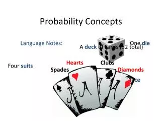
Outcome of Roll 1 2 3 4 5 6 Probability 1/6 1/6 1/6 1/6 1/6 1/6 Total = 1 Example 2 Rolling a die has six possible outcomes
Outcome of Roll = 5 Die 1 Die 2 1 4 2 3 3 2 4 1 Probability 1/36 1/36 1/36 1/36 Example 2a Rolling two dice results in a total of five spots showing. There are a total of 36 possible outcomes.
Draw a spade or a club Draw a face card or a number card Draw an ace or a 3 Draw a club or a nonclub Draw a 5 or a diamond Draw a red card or a diamond Yes No Yes Yes Yes No Yes Yes No No No No Example 3 Draw Mutually Collectively Exclusive Exhaustive
Probability : Mutually Exclusive P(event A or event B) = P(event A) + P(event B) or: P(A or B) = P(A) + P(B) i.e., P(spade or club) = P(spade) + P(club) = 13/52 + 13/52 = 26/52 = 1/2 = 50%
Probability:Not Mutually Exclusive P(event A or event B) = P(event A) + P(event B) - P(event A and event B both occurring) or P(A or B) = P(A)+P(B) - P(A and B)
P(A and B) P(A) P(B) P(A and B)(Venn Diagram)
- + P(A) P(B) P(A and B) = P(A or B) P(A or B)
Statistical Dependence • Events are either • statistically independent (the occurrence of one event has no effect on the probability of occurrence of the other) or • statistically dependent (the occurrence of one event gives information about the occurrence of the other)
Which Are Independent? • (a) Your education (b) Your income level • (a) Draw a Jack of Hearts from a full 52 card deck (b) Draw a Jack of Clubs from a full 52 card deck
Probabilities - Independent Events • Marginal probability: the probability of an event occurring: [P(A)] • Joint probability: the probability of multiple, independent events, occurring at the same time P(AB) = P(A)*P(B) • Conditional probability (for independent events): • the probability of event B given that event A has occurred P(B|A) = P(B) • or, the probability of event A given that event B has occurred P(A|B) = P(A)
P(B) P(A) P(B|A) P(A|B) Probability(A|B) Independent Events
1. P(black ball drawn on first draw) 2. P(two green balls drawn) Statistically Independent Events A bucket contains 3 black balls, and 7 green balls. We draw a ball from the bucket, replace it, and draw a second ball
1. P(black ball drawn on second draw, first draw was green) 2. P(green ball drawn on second draw, first draw was green) Statistically Independent Events - continued
Probabilities - Dependent Events • Marginal probability: probability of an event occurring P(A) • Conditional probability (for dependent events): • the probability of event B given that event A has occurred P(B|A) = P(AB)/P(A) • the probability of event A given that event B has occurred P(A|B) = P(AB)/P(B)
/ P(A) P(AB) P(B) P(A|B) = P(AB)/P(B) Probability(A|B)
/ P(B) P(AB) P(A) P(B|A) = P(AB)/P(A) Probability(B|A)
Statistically Dependent Events • Then: • P(WL) = 4/10 = 0.40 • P(WN) = 2/10 = 0.20 • P(W) = 6/10 = 0.60 • P(YL) = 3/10 = 0.3 • P(YN) = 1/10 = 0.1 • P(Y) = 4/10 = 0.4 • Assume that we have an urn containing 10 balls of the following descriptions: • 4 are white (W) and lettered (L) • 2 are white (W) and numbered N • 3 are yellow (Y) and lettered (L) • 1 is yellow (Y) and numbered (N)
Then: P(L|Y) = P(YL)/P(Y) = 0.3/0.4 = 0.75 P(Y|L) = P(YL)/P(L) = 0.3/0.7 = 0.43 P(W|L) = P(WL)/P(L) = 0.4/0.7 = 0.57 Statistically Dependent Events - Continued
Your stockbroker informs you that if the stock market reaches the 10,500 point level by January, there is a 70% probability the Tubeless Electronics will go up in value. Your own feeling is that there is only a 40% chance of the market reaching 10,500 by January. What is the probability that both the stock market will reach 10,500 points, and the price of Tubeless will go up in value? Joint Probabilities, Dependent Events
Then: P(MT) =P(T|M)P(M) = (0.70)(0.40) = 0.28 Joint Probabilities, Dependent Events - continued Let M represent the event of the stock market reaching the 10,500 point level, and T represent the event that Tubeless goes up.
Bayes’ theorem can be used to calculate revised or posterior probabilities Prior Probabilities Bayes’ Process Posterior Probabilities New Information Revising Probabilities: Bayes’ Theorem
A cup contains two dice identical in appearance. One, however, is fair (unbiased), the other is loaded (biased). The probability of rolling a 3 on the fair die is 1/6 or 0.166. The probability of tossing the same number on the loaded die is 0.60. We have no idea which die is which, but we select one by chance, and toss it. The result is a 3. What is the probability that the die rolled was fair? Posterior Probabilities
We know that: P(fair) = 0.50 P(loaded) = 0.50 And: P(3|fair) = 0.166P(3|loaded) = 0.60 Then: P(3 and fair) = P(3|fair)P(fair) = (0.166)(0.50) = 0.083 P(3 and loaded) = P(3|loaded)P(loaded) = (0.60)(0.50) = 0.300 Posterior Probabilities Continued
A 3 can occur in combination with the state “fair die” or in combination with the state ”loaded die.” The sum of their probabilities gives the unconditional or marginal probability of a 3 on a toss: P(3) = 0.083 + 0.0300 = 0.383. Then, the probability that the die rolled was the fair one is given by: Posterior Probabilities Continued
To obtain further information as to whether the die just rolled is fair or loaded, let’s roll it again. Again we get a 3. Given that we have now rolled two 3s, what is the probability that the die rolled is fair? Further Probability Revisions
P(fair) = 0.50, P(loaded) = 0.50 as before P(3,3|fair) = (0.166)(0.166) = 0.027 P(3,3|loaded) = (0.60)(0.60) = 0.36 P(3,3 and fair) = P(3,3|fair)P(fair) = (0.027)(0.05) = 0.013 P(3,3 and loaded) = P(3,3|loaded)P(loaded) = (0.36)(0.5) = 0.18 P(3,3) = 0.013 + 0.18 = 0.193 Further Probability Revisions - continued
Further Probability Revisions - continued To give the final comparison: P(fair|3) = 0.22 P(loaded|3) = 0.78 P(fair|3,3) = 0.067 P(loaded|3,3) = 0.933
Random Variables • Discrete random variable - can assume only a finite or limited set of values- i.e., the number of automobiles sold in a year • Continuous random variable - can assume any one of an infinite set of values - i.e., temperature, product lifetime
Experiment Outcome Random Variable Range of Random Variable Stock 50 Number of X = number of 0,1,2,, 50 Xmas trees trees sold trees sold Inspect 600 Number Y = number 0,1,2,…, items acceptable acceptable 600 Send out Number of Z = number of 0,1,2,…, 5,000 sales people e people responding 5,000 letters responding £ £ Build an %completed R = %completed 0 R 100 apartment after 4 after 4 months building months £ £ Test the Time bulb S = time bulb burns 0 S 80,000 lifetime of a lasts - up to light bulb 80,000 (minutes) minutes Random Variables (Numeric)
Random Variables (Non-numeric) Experiment Outcome Random Range of Variable Random Variable Students Strongly agree (SA) X = 5 if SA 1,2,3,4,5 respond to a 4 if A Agree (A) questionnaire Neutral (N) 3 if N Disagree (D) 2 if D Strongly Disagree (SD) 1 if SD One machine is Defective Y = 0 if defective 0,1 inspected Not defective 1 if not defective Consumers Good Z = 3 if good 1,2,3 respond to how Average 2 if average they like a Poor 1 if poor product
Figure 2.5 Probability Function Probability Distributions
n = å E ( X ) X P ( X ) i i = 1 i Expected Value of a Discrete Probability Distribution
Binomial Distribution Assumptions: 1. Trials follow Bernoulli process – two possible outcomes 2. Probabilities stay the same from one trial to the next 3. Trials are statistically independent 4. Number of trials is a positive integer
Binomial Distribution n = number of trials r = number of successes p = probability of success q = probability of failure Probability of r successes in n trials