Transport Layer Outline
370 likes | 556 Vues
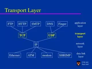
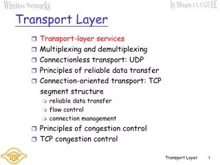
3.1 Transport-layer services 3.2 Multiplexing and demultiplexing 3.3 Connectionless transport: UDP 3.4 Principles of reliable data transfer. 3.5 Connection-oriented transport: TCP segment structure reliable data transfer flow control connection management

Transport Layer Outline
E N D
Presentation Transcript
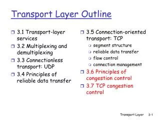
3.1 Transport-layer services 3.2 Multiplexing and demultiplexing 3.3 Connectionless transport: UDP 3.4 Principles of reliable data transfer 3.5 Connection-oriented transport: TCP segment structure reliable data transfer flow control connection management 3.6 Principles of congestion control 3.7 TCP congestion control Transport Layer Outline Transport Layer
Recap: TCP • TCP Properties: • point to point, connection-oriented, full-duplex, reliable • TCP Segment Structure • How TCP sequence and acknowledgement #s are assigned • How does TCP measure the timeout value needed for retransmissions using EstimatedRTT and DevRTT • TCP retransmission scenarios, ACK generation and fast retransmit • How does TCP Flow Control work • TCP Connection Management: 3-segments exchanged to connect and 4-segments exchanged to disconnect Transport Layer
Congestion: informally: “too many sources sending too much data too fast for network to handle” different from flow control! manifestations: lost packets (buffer overflow at routers) long delays (queueing in router buffers) a top-10 problem! Principles of Congestion Control Transport Layer
two senders, two receivers one router, infinite buffers no retransmission Cost of congested network: large queuing delays are experienced as the arrival rate nears link capacity. maximum achievable throughput is R/2 lout lin : original data unlimited shared output link buffers Host A Host B Causes/costs of congestion: scenario 1 link is shared between 2 connections/senders and that is the why the maximum transmission rate is R/2 where R is the capacity of the link Transport Layer
one router, finite buffers sender retransmission of lost packet (but actually delayed packet) with 3 possible sub-scenarios Causes/costs of congestion: scenario 2 Host A lout lin : original data l'in : original data, plus retransmitted data Host B finite shared output link buffers Transport Layer
a) (assume sender only sends pkts when router’s buffer is free, no packets are lost) b) sender retransmit only when packets are known to be lost (large timeout): Out of 0.5R data transmitted, 0.33R average are original data and 0.16R are retransmitted c) retransmission of delayed (not lost) packet makes larger (premature timeout): For every 0.5R data transmitted, 0.25R average are original data and 0.25R are retransmitted since for every delayed packet another packet is resent. l l = > l l R/2 l l in in in in R/2 R/2 out out R/3 lout lout lout R/4 R/2 R/2 R/2 lin lin lin a. b. c. Causes/costs of congestion: scenario 2 = offered load is the rate that transport layer sends segments with original and retransmitted data to the network “costs” of congestion: • sender performs retrans to compensate for dropped/lost packets due to buffer overflow • unneeded retransmissions by sender causes router to forward multiple copies of pkt Transport Layer
four senders overlapping 2-hop paths timeout/retransmit to implement RDT service all senders have similar transmission rates l l Q:what happens as and increase ? in in Causes/costs of congestion: scenario 3 Transport Layer
Causes/costs of congestion: scenario 3 As sending rates increases, routers farther away will be busy sending pkts for closer senders Another “cost” of congestion: • a dropped packet on the 2nd router causes 1st router work to be wasted. It would have been better if the 1st router dropped it. • when packet dropped, any “upstream transmission capacity used for that packet was wasted! • decrease in throughput with increased offered load Transport Layer
End-end congestion control: no explicit feedback from network congestion inferred from end-system observed loss, delay approach taken by TCP: timeout or triple duplicate ACKs are indications of network congestion Network-assisted congestion control: routers provide feedback to end systems single bit indicating congestion (SNA, DECbit, TCP/IP ECN, ATM) explicit rate supported by router that sender should send at Approaches towards congestion control Two broad approaches towards congestion control: Transport Layer
ABR: available bit rate: “elastic service” if sender’s path “underloaded”: sender should use available bandwidth if sender’s path congested: sender throttled to minimum guaranteed rate RM (Resource Management) cells: sent by sender, interspersed with data cells (default rate of 1 RM/32 data cells) bits in RM cell set by switches (“network-assisted”) NI bit: no increase in rate (mild congestion) CI bit: congestion indication RM cells returned to sender by receiver, with bits intact except for the CI bits. Case study: ATM ABR congestion control ATM=Asynchronous Transfer Mode Transport Layer
two-byte ER (Explicit Rate) field in RM cell congested switch may lower ER value in cell sender’ send rate thus minimum supportable rate on path across all switches EFCI (Explicit Forward Congestion Indication) bit in data cells: set to 1 in congested switch to indicate congestion to destination host. when RM arrives at destination, if most recently received data cell has EFCI=1, sender sets CI bit in returned RM cell Case study: ATM ABR congestion control Transport Layer
3.1 Transport-layer services 3.2 Multiplexing and demultiplexing 3.3 Connectionless transport: UDP 3.4 Principles of reliable data transfer 3.5 Connection-oriented transport: TCP segment structure reliable data transfer flow control connection management 3.6 Principles of congestion control 3.7 TCP congestion control Transport Layer Transport Layer
1) How does TCP sender limit the sending rate ? 2) How does TCP sender know that there is network congestion ? 3) What algorithm sender uses to change its rate as a function of the network congestion ? “TCP Reno” congestion control algorithm is used in most OSs. TCP Congestion Control Transport Layer
end-end control (no network assistance) Sender limits transmission rate to (LastByteSent-LastByteAcked) min {CongWin, RcvWin} Assuming a very large RcvWin, this limits amount of unACKed data (LastByteSent-LastByteAcked) to CongWin and therefore limits sender send rate: CongWin is dynamic, function of perceived network congestion How does sender perceive congestion? loss event = timeout or 3 duplicate acks TCP sender reduces rate (CongWin) after loss event TCP is said to be self-clocking because it uses ACKs to trigger(clock) its increase in CongWin size. three components: AIMD slow start conservative after timeout events CongWin rate = Bytes/sec RTT TCP Congestion Control Transport Layer
multiplicative decrease: cut CongWin in half after loss event (timeout or 3 ACKs for same segment) until CongWin = 1 MSS. TCP AIMD (Additive-Increase, Multiplicative-Decrease) additive increase: • increase CongWin by 1 MSS every RTT in the absence of loss events: cautiously probing for additional available bandwidth in the end-to-end path. • Congestion Avoidance is the linear increase phase of the TCP congestion control protocol. • Example: if MSS=1 Kbyte and CongWin=10 Kbytes, 10 segments are sent within 1 RTT, each arriving ACK (one ACK per segment) increases CongWin size by 1/10 MSS and by 1 MSS after all 10 ACKs are received. Long-lived TCP connection, CongWin increases linearly and suddenly drops to half its size when a loss event occurs Transport Layer
When connection begins, CongWin = 1 MSS Example: MSS = 500 bytes & RTT = 200 msec initial rate = 20 kbps available bandwidth may be >> MSS/RTT desirable to quickly ramp up to respectable rate TCP Slow Start • When connection begins, increase rate exponentially fast until first loss event Transport Layer
When connection begins, increase rate exponentially until first loss event: double CongWin every RTT done by incrementing CongWin by 1 MSS for each ACKed segment Summary: initial rate is slow but ramps up exponentially fast time TCP Slow Start (more) Host A Host B one segment RTT two segments four segments Transport Layer
introduce a new variable called Threshold initially set to a high value (65 kbytes in practice) After 3 duplicate ACKs event: set Threshold = CongWin/2 just before event set CongWin = Threshold window then grows linearly But after timeout event: set Threshold = CongWin/2 just before timeout event set CongWin = 1 MSS CongWin window grows exponentially to the Threshold value using the Slow Start SS algorithm, then grows linearly as in the Congestion Avoidance phase. Refinement for timeout events Philosophy: * 3 dup ACKs indicates network capable of delivering some segments. * Timeout, before 3 dup ACKs, is “more alarming” The canceling of the Slow Start SS phase after 3 duplicate ACKs is called fast recovery Transport Layer
Summary: TCP Congestion Control • When CongWin is below Threshold, sender in slow-start SS phase, window grows exponentially. • When CongWin is above Threshold, sender is in congestion-avoidance phase, window grows linearly. • When a triple duplicate ACK occurs, Threshold set to CongWin/2 and CongWin set to Threshold. • When timeout occurs, Threshold set to CongWin/2 and CongWin is set to 1 MSS. • New proposed TCP Vegas algorithm: • detect network congestion before packet loss occurs. • imminent packet loss is predicted by observing the RTT of segments where increasing RTTs indicates increasingly congested routers. • lower send rate linearly when this imminent packet loss is detected. Transport Layer
TCP sender congestion control Transport Layer
TCP throughput • What’s the average throughout of TCP (bps) as a function of window size and RTT? • Ignore slow start • Let W be the window size when loss occurs. • When window is W, throughput is W/RTT which is the max send rate before a loss event. • Just after loss, window drops to W/2, throughput to W/2RTT. • Average throughout: 0.75 W/RTT Transport Layer
TCP Futures • Example: 1500 byte segments, 100ms RTT, want 10 Gbps throughput • Requires window size W = 83,333 in-flight segments to achieve this max rate • Throughput in terms of loss rate (the ratio of the number of packets lost over the number of packets sent): • To achieve a throughput of 10 Gbps, today’s TCP congestion control algorithm can only tolerate a segment loss probability of L = 2 *10-10 or one loss event for every 5 Billion segments. • New versions of TCP for high-speed internet needed! Transport Layer
TCP Throughput as a function of loss rate L, MSS and RTT Transport Layer
Fairness defined: if K TCP sessions share same bottleneck link of bandwidth R, each should have average transmission rate of R/K. In other words, each connection gets an equal share of the link bandwidth. TCP connection 1 bottleneck router capacity R TCP connection 2 TCP Fairness Transport Layer
Two competing sessions: Assume both have the same MSS and RTT so that if they have the same CongWin size then they have the same throughput. Assume both have large data to send and no other data traverses this shared link. Assume both are in the CA state (AIMD) and ignore the SS state. Additive increase gives slope of 1, as throughout increases multiplicative decrease decreases throughput proportionally Why is TCP fair? * If connections 1&2 are at point A then the joint bandwidth < R and both connection increase their CongWin by 1 until they get to B where the joint bandwidth > R and loss occur and CongWin is decreased by half to point C (point C is the middle of the line from B to zero). * Bandwidth realized by the 2 connections fluctuates along the Equal bandwidth share line. * It has been shown that when multiple sessions share a link, sessions with smaller RTT are able to open their CongWin faster and hence grab available bandwidth at that link faster as it becomes free. As a result those sessions enjoy a higher throughput than sessions with larger RTTs. Transport Layer
Fairness and UDP Multimedia apps often do not use TCP do not want rate throttled by congestion control Instead use UDP: pump audio/video at constant rate, tolerate packet loss Research area: develop congestion control for the Internet to prevent UDP from dramatically affecting the throughput. Fairness and parallel TCP connections nothing prevents app from opening parallel connections between 2 hosts. Web browsers do this Example: link of rate R supporting 9 connections; new app asks for 1 TCP, gets rate R/10 new app asks for 11 TCPs, gets R/2 ! Fairness (more) Transport Layer
Q:How long does it take to receive an object from a Web server after sending a request? Latency is the time the client when initiates a TCP connection until receiving the complete object. Key components of Latency are: 1) TCP connection establishment, 2) data transmission delay, 3) slow start Notation, assumptions: one link between client and server of rate R amount of sent data depends only on CongWin (large RcvWin) all protocols headers and non-file segments are ignored file send has integer number of MSSs large initial Threshold no retransmissions (no loss, no corruption) MSS is S bits object size is O bits R bps is the transmission rate Latency lower bound with no congestion window constraint = 2RTT (TCP Conn) + O/R Congestion Window size: First assume: fixed congestion window, W segments Then dynamic window, modeling slow start Delay modeling Transport Layer
First case: WS/R > RTT + S/R: server receives ACK for 1st segment in 1st window before 1st window’s worth of data sent where W=4. Segments arrive periodically from server every S/R seconds and ACKs arrive periodically at server every S/R seconds Fixed congestion window (1) delay = 2RTT + O/R Transport Layer
Second case: WS/R < RTT + S/R: server waits for ACK after sending all window’s segments where W=2. Fixed congestion window (2) delay = 2RTT + O/R + (K-1)[S/R + RTT - WS/R] * K = # windows of data that cover the object or K=O/WS * Additional stalled state time between the transmission of each of the windows. For K-1 periods (server not stalled when transmitting last window ) with each period lasting RTT-(W-1)S/R Transport Layer
TCP Delay Modeling: Slow Start (1) Now suppose window grows according to slow start Will show that the delay for one object is: where P is the number of times TCP idles at server: - where Q is the number of times the server idles if the object were of infinite size. - and K is the number of windows that cover the object. Transport Layer
TCP Delay Modeling: Slow Start (2) • Delay components: • 2 RTT for connection estab and request • O/R to transmit object • time server idles due to slow start • Server idles: P =min{K-1,Q} times • Example: • O/S = 15 segments in object • K = 4 windows • Q = 2 • P = min{K-1,Q} = 2 • Server idles P=2 times Transport Layer
TCP Delay Modeling (3) Transport Layer
TCP Delay Modeling (4) Recall K = number of windows that cover object How do we calculate K ? Calculation of Q, number of idles for infinite-size object, is similar. TCP Slow Start can significantly increase latency when object size is relatively small and the RTT is relatively large which is the case with the Web. Transport Layer
HTTP Modeling • Assume Web page consists of: • 1 base HTML page (of size O bits) • M images (each of size O bits) • Non-persistent HTTP: • M+1 TCP connections in series • Response time = (M+1)O/R + (M+1)2RTT + sum of idle times • Persistent HTTP with pipelining: • 2 RTT to request and receive base HTML file • 1 RTT to request and receive M images • Response time = (M+1)O/R + 3RTT + sum of idle times • Non-persistent HTTP with X parallel connections • Suppose M/X integer (high chance that M=X). • 1 TCP connection for base file • M/X sets of parallel connections for images. • Response time = (M+1)O/R + (M/X + 1)2RTT + sum of idle times Transport Layer
HTTP Response time (in seconds) RTT = 100 msec, O = 5 Kbytes, M=10 and X=5 For low bandwidth, connection & response time dominated by transmission time. Persistent connections only give minor improvement over parallel connections. Transport Layer
HTTP Response time (in seconds) RTT =1 sec, O = 5 Kbytes, M=10 and X=5 For larger RTT, response time dominated by TCP establishment & slow start delays. Persistent connections now give important improvement: particularly in high delay and bandwidth networks. Transport Layer
Reasons and Symptoms of Network Congestion There are 2 Congestion Control Approaches ATM Available Bit Rate (ABR) Congestion Control TCP Congestion Control 3 mechanisms: Additive-Increase, Multiplicative-Decrease (AIMD) algorithm Slow Start algorithm Conservative after timeout events algorithm TCP Throughput as a function of window size and RTT TCP Futures and why new versions of TCP needed for high speed networks TCP Fairness vs UDP and TCP with parallel connections TCP Delay Modeling HTTP Delay and Response Time Summary Transport Layer