### River Water Level Prediction Using Satellite-based Microwave Signatures ###
160 likes | 292 Vues
This workshop addresses the development of a river water level prediction model utilizing passive microwave signatures, specifically Brightness Temperature (TB) data from AMSR-E and SMOS satellite acquisitions. The study focuses on the Lower Bermejo Basin in Argentina, which is prone to severe flooding events. By combining satellite data with hydrometric and rainfall measurements, this research explores the relationship between precipitation, vegetation, and flooding dynamics. The results aim to enhance flood risk management and enable accurate forecasting for agriculture and energy production. ###

### River Water Level Prediction Using Satellite-based Microwave Signatures ###
E N D
Presentation Transcript
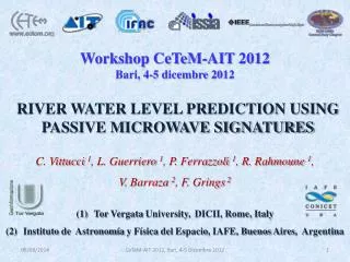
Workshop CeTeM-AIT 2012 Bari, 4-5 dicembre 2012 RIVER WATER LEVEL PREDICTION USING PASSIVE MICROWAVE SIGNATURES C. Vittucci1, L. Guerriero 1, P. Ferrazzoli1, R. Rahmoune1, V. Barraza2, F. Grings 2 Tor Vergata University, DICII, Rome, Italy Institutode Astronomíay Física del Espacio, IAFE, Buenos Aires, Argentina CeTeM-AIT 2012, Bari, 4-5 Dicembre 2012
Summary • Objective: • To investigate the exploitation of satellite acquisitions of Brightness Temperature (TB) for the prediction of river water level. • To develop a useful forecast model using ground and satellite observations. • Hypothesis: • Passive sensors sensitivity to short term variations of TB after rainfall or floodingalso in presence of vegetation during different seasons. • soilsurface antecedentconditions • Relationship betweenflooding and: infiltration capacity • local and upper basin rainfalls • Tools: • AMSR-E(at C, X, Ka Bands) and SMOS (L Bands) + hydrometric and rainfall ground measurements. • Temporal Range: • 2010-2011observations datasets. • Case Study: • LowerBermejo Basin, northen Argentina, seasonally affected by severe flooding events. CeTeM-AIT 2012, Bari, 4-5 Dicembre 2012
The Bermejo Basin Area: [-22 ; -27 S] Lat and [-58; -66 W] Lon, about123,000km2 Climate: Continental, subtropical characteristics Lower basin vegetation: Rain forest, humid valley, gallery forest moderately dense Study Area: Humid Chaco, dominated by a typical tree species Schinopsisbalansaein the North,grasslandin the South. ElSauzalito Hydrometric Station Rainfall Station El Colorado Puerto Bermejo Laguna Limpia GralVedia Mapped area CeTeM-AIT 2012, Bari, 4-5 Dicembre 2012
AMSR-E C Band emissivitymaps SMOS –L Band emissivity maps AMSR-E X Band emissivitymaps [-27 -25 Lat S; -60 -58 Lon W] epf= TBpf/Ts* epf= TBpf/Ts AMSR-E emissivity: AMSR-E Ts: SMOS emissivity: Ts= 0,94 TBv(ka) + 30,8 *Ts extracted from ECMWF auxiliary products. (a) NormalCondition (b) RainCondition (c) FloodingCondition CeTeM-AIT 2012, Bari, 4-5 Dicembre 2012
HydrometricStationsInvolved 2010 – 2011 ElSauzalitodailyobservationsofriver water level 2010 – 2011 El Colorado dailyobservationsofriver water level Rainy Season Rainy Season Dry Season Dry Season CeTeM-AIT 2012, Bari, 4-5 Dicembre 2012
Emissivity at C Band and Rain Trend Emissivity at L Band and Rain Trend Emissivity at X Band and Rain Trend Rainy Season Rainy Season Rainy Season Rainy Season Rainy Season Rainy Season Dry Season Dry Season Dry Season Dry Season Dry Season Dry Season CeTeM-AIT 2012, Bari, 4-5 Dicembre 2012
Adaptive Filter theory Daily Satellite + ground data asINPUTof LINEAR ADAPTIVE FILTER* Weightschange with time to minimizethe errorhere between the model output and ground truth. L= Lag time, forecasthorizon y(t+L) = ŵ(t)x(t) y(t): filter output, i.e., predicted Water Level WL at El Colorado Station w(t): weight vector x(t) : input signal * Haykin, “AdaptiveFilterTheory” , 2001 CeTeM-AIT 2012, Bari, 4-5 Dicembre 2012
FloodForecastingInputs Legend Pn(i)= Precipitation at t time occurred in the nthstation (n=1, 2,3,4) WL ElS(i) = ElSauzalito Water Level at t time e Bpf(i) = Emissivity values for both polarizations at C, X, Ka, L bands, averaged over (0.5 x 0.5 deg) area B = number of days backward with respect to the actual day t. (In our study B=7 days before t time) i = t - B+1, t P1(i), GralVedia P2 (i), Puerto Bermejo P3 (i), El Colorado P4 (i),Laguna Limpia WL ElS(i), ElSauzalito AQUA AMSR-E or SMOS MIRAS e BvC(i), eBhC(i), e BvX(i), e BhX(i), eBvL(i),e BhL(i) eBvKa(i), e BhKa(i), GROUND INPUT X(t) SATELLITE INPUT CeTeM-AIT 2012, Bari, 4-5 Dicembre 2012
Water LevelForecastingAlgorithm L = lag time, heretested for L=3; L=5; L=7 days Y(t+L) = W(t)TX(t) X(t)is updated with the new incoming data and contains the information acquired from day t-B+1tot. R(t): Residual error R(t) = WL(t) – Y(t)Y(t):water level prediction at time t WL(t): WL observed at El Colorado Station Residual is computed at each step to adjust the vector of weights applying the following formula: W(t+1)= W(t) + µ X(t-L) R(t) to minimise residualerror. µ= step size parameter. CeTeM-AIT 2012, Bari, 4-5 Dicembre 2012
Results : Observed and PredictedTrendsof Water Level L = 3 L = 7 CeTeM-AIT 2012, Bari, 4-5 Dicembre 2012
Results: Predicted vs. Observed L=3 L=5 L=7 CeTeM-AIT 2012, Bari, 4-5 Dicembre 2012
Inputs : Ground measurements NO Microwaveradiometric data as INPUTS ALGORITHM TEST To prove the effectivenessof satellite information L=3 L=7 CeTeM-AIT 2012, Bari, 4-5 Dicembre 2012
FloodForecastingStatistics Tab 2. RMSE and R2 for each Lead time for both sensors (e case) CeTeM-AIT 2012, Bari, 4-5 Dicembre 2012
Conclusions SMOS or AMSR-E + Rainfall and upstream water level Successfull InputsTogether Adaptivealgorithm Water LevelPrediction Sensitivity to surface conditions Accurate Prediction (best for L=3) • Realapplications • FloodingRisk Management • Agriculture • Electricity Production ForecastHorizons: L=3; L=5; L=7 Simultaneouslyapplied • Over Target • No assumptions • No costraints CeTeM-AIT 2012, Bari, 4-5 Dicembre 2012
Workshop CeTeM-AIT 2012 Bari, 4-5 dicembre 2012 THANKS FOR YOUR ATTENTION CONTACT: vittucci@disp.uniroma2.it CeTeM-AIT 2012, Bari, 4-5 Dicembre 2012