Download
1 / 36
360 likes | 568 Vues
Satellite-based Estimation of Precipitation Using Passive Opaque Microwave Radiometry*. Frederick W. Chen, Laura J. Bickmeier, William J. Blackwell, R. Vincent Leslie MIT Lincoln Laboratory (Lexington, MA, USA) David H. Staelin, Chinnawat “Pop” Surussavadee

E N D
Satellite-based Estimation of PrecipitationUsing Passive Opaque Microwave Radiometry* Frederick W. Chen, Laura J. Bickmeier, William J. Blackwell, R. Vincent Leslie MIT Lincoln Laboratory (Lexington, MA, USA) David H. Staelin, Chinnawat “Pop” Surussavadee MIT Research Laboratory of Electronics (Cambridge, MA, USA) 3rd Workshop of the International Precipitation Working Group Melbourne, VIC, Australia 24 October 2006 * This work was sponsored by the National Aeronautics and Space Administration under Contract NNG 04HZ53C, Grant NNG 04HZ51C, and Grant NAG5-13652, and the National Oceanic and Atmospheric Administration under Air Force Contract FA8721-05-C-0002. Opinions, interpretations, conclusions, and recommendations are those of the author and are not necessarily endorsed by the United States Government.
Outline • Physical basis • Algorithm development • AMSU (Advanced Microwave Sounding Unit) • ATMS (Advanced Technology Microwave Sounder) • Future work • Summary
Physical Basis • Transparent channels (or window channels) • Warm water vapor signatures over cold ocean • Scattering signatures due to ice particles over land • Opaque channels • Varying atmospheric opacity • Sensitive primarily to specific layers of atmosphere OPAQUE BANDS TRANSPARENT BANDS
54-GHz and 183-GHz Weighting Functions 54-GHz 183-GHz
Estimation of Precipitation Rate with Opaque W Channels(54-GHz and 183-GHz) • Precipitation rate ~ humidity × vertical wind velocity • Absolute humidity • 54-GHz band revealtemperature profile • 54-GHz and 183-GHz bands reveal water vapor profile • Vertical wind velocity • Stronger vertical wind → • Stronger vertical winds results in increased backscattering of cold space radiation • Perturbations (cold spots) in 54-GHz data reveal cloud-top altitude • Absolute albedos reveal hydrometeor abundance • Relative albedos (54 vs. 183-GHz) reveal hydrometeor size Greater hydrometeors size Greater hydrometeor abundance Higher cloud-top altitude
Particle Sizes Revealed in NAST-M Data 54 GHz 118 GHz TB 183 GHz 425 GHz Visible Leslie & Staelin, IEEE TGRS, 10/2004
AMSU Radiometry • Passive W sounder • AMSU-A • 12 channels in opaque 54-GHz O2 band • Window channels near 23.8, 31.4, and 89.0 GHz • AMSU-B • 3 channels in opaque 183.31-GHz H2O band • Window channels near 89.0 and 150.0 GHz
General Structure of AMSU Algorithm(Chen and Staelin, IEEE TGRS, 2/2003) • Signal processing • Regional Laplacian interpolation • Image sharpening • Principal component analysis • Neural net • 2-layer feedforward neural net • 1st layer: tanh transfer function • 2nd layer: linear transfer function
Signal Processing Components • Neural-net correction of angle-dependent variations in TB’s • Cloud-clearing via regional Laplacian interpolation • Temperature profile characterization • Cloud-top altitude characterization • Principal component analysis for dimensionality reduction • Temperature profile PC’s • Window channel / H2O profile PC’s • Image sharpening • AMSU-A data sharpened to AMSU-B resolution
The Algorithm: Precipitation Masks &Precipitation-Induced Perturbations IMAGE SHARPENING PRECIPITATION DETECTION CORRUPT DATA DETECTION LIMB-&-SURFACE CORRECTION REGIONAL LAPLACIAN INTERPOLATION
The Algorithm: Neural Net Trained to NEXRAD
ATMS • Similar to AMSU • To be launched on NPP (2009) & NPOESS satellites • NPP = NPOESS Preparatory Project • Improvements over AMSU • Additional channels in 54-GHz and 183-GHz bands • Better resolution in 54-GHz band • Better sampling • Nyquist sampling of 54-GHz data • Identical sampling of all channels
Simulating ATMS TB’s • MM5 Atmospheric Circulation Model • Provides temperature profile, water vapor profile, hydrometeor profile, … • Used Goddard hydrometeor model (Tao & Simpson, 1993) • Radiative Transfer • TBSCAT due to Rosenkranz (IEEE TGRS, 8/2002) • Multi-stream, initial-value • Improved hydrometeor modeling due to Surussavadee & Staelin (IEEE TGRS, 10/2006) • Filtering • Accurate matching of TB’s on MM5 grid to ATMS resolution and geolocation using “satellite geometry” toolbox for MATLAB • Computing angular offset of surface locations from boresight • Computing satellite zenith angles from scan angle • Computing geolocation from scan angle
AMSU vs. ATMS, 183±7 GHz Observed AMSU Simulated ATMS • Simulated ATMS 183±7 GHz data shows reasonable agreement with AMSU-B • Morphology difference between AMSU observations and MM5 predicted radiances is due to the inaccuracy of the NCEP analyses used to initialize the MM5 model
AMSU vs. ATMS, 50.3 GHz Observed AMSU Simulated ATMS • Simulated ATMS 50.3-GHz data with finer resolution and sampling shows finer features than AMSU-A • Intense eyewall signature in simulated ATMS 50.3-GHz data due to NCEP initialization & limited 5-hr MM5 spinup time producing excess of large ice particles
Future Developments • Adapting Chen-Staelin algorithm (IEEE TGRS, 2/2003) for ATMS • Exploiting Nyquist sampling in the 54-GHz band • Using methods from window-channel-based algorithms • Improving the signal processing of Chen-Staelin algorithm • Improving neural net training • Representations of circular data
Recently Launched & Future Instruments • Similar to AMSU-A/B • AMSU/MHS on NOAA-18 (2005) • AMSU/MHS on NOAA-N’, METOP-1, METOP-2, METOP-3 • ATMS • NPP (2009) • NPOESS • W instruments on geostationary satellites? • < 1 hr revisit times
Summary • Physical basis of precipitation estimation using opaque W channels • Atmospheric sounding capabilities of opaque W channels • Cloud shape and particle size distribution from NAST-M 54-, 118-, 183-, and 425-GHz data • AMSU precipitation algorithm • Relies primarily on 54-GHz and 183-GHz opaque bands • Signal processing: regional Laplacian interpolation, principal component analysis, image sharpening • ATMS precipitation algorithm development • Simulation system using MM5/TBSCAT
NAST-M • NAST = NPOESS Aircraft Sounder Testbed • Risk-reduction effort by NPOESS Integrated Program Office • Cooperative effort of NASA, NOAA, & DoD • Equipped with 54-, 118-, 183-, and 425-GHz radiometers • Flown on high-altitude aircraft • ER-2 (NASA) • Proteus (Scaled Composites) • ~2.5-km resolution near nadir
Scattering in the 54-GHz and 183-GHz Bands 0.7 mm 2.4 mm
AMSU Geographical Coverage • Aboard NOAA-15, NOAA-16, & NOAA-17 • Nearly identical AMSU/HSB on Aqua
AMSU-A/B Sampling & Resolution AMSU-A AMSU-B • AMSU-A • 3 1/3° sampling (~50 km near nadir) • 3.3° resolution (~50 km near nadir) • AMSU-B • 1.1° resolution (~15 km near nadir) • 1.1° sampling (~15-km near nadir)
Features of ATMS vs. AMSU • Channel set • Similar to AMSU • Additional 51.76-GHz channel • Additional 183.31±4.5-GHz & 183.31±1.8-GHz • 165.5-GHz replaces 150-GHz on AMSU-B • No 89.0-GHz 15-km channel (available on AMSU-B) • Resolution • 54-GHz and 89-GHz: 2.2° vs. 3.33° on AMSU • 23.8- and 31.4-GHz: 5.2° vs. 3.33° on AMSU • Sampling • 165.5-GHz, 183-GHz: Similar to AMSU-B • Other channels: ~3× finer than AMSU-A cross-track & along-track • All channels sampled at the same locations • Nyquist sampling of 54-GHz and 89-GHz • Similar sensitivity
ATMS Rain Rate Retrieval Algorithm • Completely new algorithm • Neural net • Inputs • All 22 channels • sec(satellite zenith angle) • Training, validation, and testing sets • MM5 data over Typhoon Pongsona • 1 time step (1521 data points) each for training, validation, and testing
Representations of Geolocation Rectangular (2-D) • Discontinuity across 180° E/W (Int’l Date Line) • Topological distortion around 90° N & 90° S (Geo. N & S Poles) Cylindrical (3-D) • Continuity across 180° E/W • Topological distortion around 90° N & 90° S Spherical (3-D) • Continuity across 180° E/W • No topological distortion around 90° N & and 90° S
Geolocation:Comparing the Representations • Spherical representation produces the lowest RMS errors • RMS error with 10 weights & biases • Linear: 0.16 • Cylindrical: 0.16 • Spherical: 0.01 • Weights & biases needed for RMS error < 1.5 × 10⁻² • Rectangular: 23 • Cylindrical: 18 • Spherical: 6 RECTANGULAR CYLINDRICAL SPHERICAL