8 - Introduction to Two-Dimensional NMR Spectroscopy
1.22k likes | 3.01k Vues
8 - Introduction to Two-Dimensional NMR Spectroscopy. 1. Introduction 2. Heteronuclear (C,H) Correlation 3. HETCOR and COLOC 4. Summary. Introduction: Why two-dimensional NMR?.

8 - Introduction to Two-Dimensional NMR Spectroscopy
E N D
Presentation Transcript
8 - Introduction to Two-Dimensional NMR Spectroscopy 1. Introduction 2. Heteronuclear (C,H) Correlation 3. HETCOR and COLOC 4. Summary
08-Introduction to 2-D NMR (Dayrit) Introduction: Why two-dimensional NMR? • Neighboring nuclei interact with each other through bonding electrons or through space by direct dipole-dipole interaction. We can elucidate these interactions using double-irradiation experiments, such as decoupling of J-multiplets and NOE. • When we perform double irradiation experiments, we perform separate experiments to irradiate each nucleus of interest. This method is conveniently done if one is interested only in a few nuclei, and is impractical or not feasible for an entire molecule. • Two-dimensional NMRis essentially an algorithmic way of accomplishing double resonance experiments.
08-Introduction to 2-D NMR (Dayrit) Introduction Two-dimensional NMR pulse sequences can be divided into four parts: preparation, evolution, t1, mixing, m, and detection, t2. t1 t2 prepn. m PD
08-Introduction to 2-D NMR (Dayrit) t1 t2 prepn. m PD • Preparation: • As in the 1-D NMR case, the objective of the preparation stage is to put the system in steady-state equilibrium. Evolution, t1: • The 2-D NMR experiment systematically varies a time period, designated as t1, from 0 seconds, increasing in fixed increments, to a pre-selected maximum value. This allows the spin information to evolve according to t1. • Since t1 is varied systematically, we are able to “map out” the evolution of the transfer of information among the spins.
08-Introduction to 2-D NMR (Dayrit) t1 t2 prepn. m PD Mixing time, m: • The mixing time, m, allows the spin information that is generated during the evolution time to spread out through the spin system. • Detection, t2: • A separate FID is acquired in t2 for each t1 value. This is Fourier-transformed as the first FID. A second FT is performed to process t1. • The two FT operations convert the time-domain data (t1 and t2) into frequency data, F1 and F2 (or 1 and 2). This is referred to as a double Fourier transform.
08-Introduction to 2-D NMR (Dayrit) Illustration of Double Fourier Transformation Process In a 2-D NMR experiment, we have two sets of FIDs which are collected representing t2 (detection) and t1 (the time increment). Two FT operations are performed, the first one on t2. (t1, t2) (t1, F2) (F1, F2) FT1 FT2 (Sanders and Hunter, Modern NMR Spectroscopy.)
Illustration of Double Fourier Transformation Process (t1, t2) (t1, F2) (F1, F2) (a) Each t1 increment (column point) yields an FID. There is a real and an imaginary part representing the sine and cosine components. (b) The first FT converts t2 to F2. (c) The real and imaginary parts are transposed. The slices trace an FID when viewed along t1. (d) The second FT converts t1 to F1. The result is a 2-dimensional spectrum: (F1, F2). FT1 FT2
08-Introduction to 2-D NMR (Dayrit) The 2-D Spectrum Double FT yields a “stack plot” which shows the individual traces along t1. Since a stack plot with many peaks is difficult to read, the contour plot is generally used. The peaks may be integrated to give the strength of the correlation. Contour plot Stack plot (from Derome)
08-Introduction to 2-D NMR (Dayrit) Two-dimensional Homonuclear NMR A 2-D homonuclear NMR experiment observes the correlations between the same types of nuclei, most commonly, 1H - 1H. The most important examples of 2-D homonuclear experiments are cosy and noesy. t1 t2 prepn. m PD 1H
08-Introduction to 2-D NMR (Dayrit) The Homonuclear 2-D Spectrum A homonuclear 2-D NMR experiment yields a symmetrical spectrum where both the x- and y-axes cover the same frequencies. t2F2 0 ppm 0 ppm • One needs to read only half of the off-diagonals. • The diagonal contains self-correlation signals and is not useful. In fact, pulse sequences are designed to minimize its intensity. off-diagonal t1F1 diagonal
08-Introduction to 2-D NMR (Dayrit) Frequency channels in NMR Instrumentation The various nuclei are observed at different Larmor frequencies. Modern NMRs are designed as multi-channel instruments, with 2 to as many as 4 channels. A basic 2-channel NMR instrument has a “high frequency” channel for irradiation and detection of 1H and 19F, and a “low frequency” channel for irradiation and detection of all other nuclei. In addition, there is “lock channel” dedicated for 2H.
08-Introduction to 2-D NMR (Dayrit) Frequency channels in NMR Instrumentation • The probe is designed according to the number of channels available. A 2-channel system uses a probe with two coils, a HF coil and a LF coil, plus a 2H lock coil. • There are two coil configurations: a standard probe (e.g., TH5) where the LF coil is placed closer to the NMR tube, and an “inverse probe” where the HF coil is closer the NMR tube. The probes are used according to the nucleus being detected. LF HF HF LF NMR tube NMR tube Inverse probe Standard probe
08-Introduction to 2-D NMR (Dayrit) Two-Dimensional Heteronuclear NMR Two-dimensional heteronuclear NMR requires a two-channel instrument where the high-frequency channel is set for 1H and the low-frequency channel can set for a nucleus of lower , such as 13C, 15N, or other nucleus of interest. The generalized pulse sequence is divided into the four parts: preparation, evolution, t1, mixing, m, and detection, t2. Detection can be set for either nucleus (channel). t1 t2 prepn. m PD (A 1H detecting expt requires an inverse probe.) 1H irr. 13C
08-Introduction to 2-D NMR (Dayrit) The Heteronuclear 2-D Spectrum: The heteronuclear 2-D NMR experiment gives a spectrum where both the x-axis if assigned as F2, while the y-axis is F1. Since the axes represent different nuclei, the spectrum is not symmetric. t2F2 (1H) 10 ppm 0 ppm t1F1 (13C) 200 ppm 0 ppm
08-Introduction to 2-D NMR (Dayrit) The 2-D Advantage 2-D NMR gives two important advantages: • First, the problem of overlapping signals is minimized. There are more data points giving greater overall resolution. For example, a typical 1-D spectrum has 16k points vs. the corresponding 2-D spectrum with 1024 pt/increment x 512 increments = 524k points. • Second, the systematic increment of the evolution time, t1, in a 2-D experiment is the equivalent of many separate 1-D experiments. The idea behind 2-D NMR spectroscopy is actually simple: to systematically modulate the evolution of a magnetization transfer process during t1.
08-Introduction to 2-D NMR (Dayrit) The 2-D Advantage • Consider a homonuclear or heteronuclear decoupling experiment. In principle, if one had lots of time, one can carry out decoupling comprehensively by moving the CW decoupling frequency across the entire spectrum giving many separate 1-D spectra. If we line up these spectra according to the position of the CW irradiation frequency, one “dimension” will be the frequency scale while the second “dimension” will be the position of the CW irradiation frequency. • COSY and HETCOR can be considered as the equivalent to these CW decoupling experiments. In addition, the 2-D NMR pulse sequence seeks to carry out all of these separate measurements in one experiment in a fraction of the time.
08-Introduction to 2-D NMR (Dayrit) Anatomy of the HETCOR pulse sequence 1H: 90x’ - t1 - 90x’ . . . . . . . . . . . 13C: . . . . . t1 - 90x’ - AQT(t2) (from: Jacobsen, NMR Spectroscopy Explained)
08-Introduction to 2-D NMR (Dayrit) Heteronuclear (C,H)-Correlation 1H: 90x’ - t1 - 90x’ . . . . . . . . . . . 13C: . . . . . t1 - 90x’ - AQT(t2) Behavior of a 1H singlet vector in the (90x’ - t1 - 90x’) sequence of HETCOR. In this illustration, t1 = 1/JCH. For intermediate values of t1 the second pulse will act only on the y’- component of vector. Polarization transfer of the 1H spin population to 13C occurs after the second pulse. (from: Sanders and Hunter, Modern NMR Spectroscopy)
Heteronuclear (C,H)-Correlation A. Pulse sequence. B. Evolution of the 1H vectors MHC and MHC for a two-spin 1H-13C system. Diagrams (d-e) show the behavior of MHC while (f-g) are for MHC. Diagram (h) shows the 1H vectors immediately before the 13C 90°x’ pulse. Only the ±z components contribute to polarization transfer to 13C. (from: Friebolin, Basic One- and Two-Dimensional NMR Spectroscopy)
08-Introduction to 2-D NMR (Dayrit) Heteronuclear (C,H)-Correlation 1H: 90x’ - t1 - 90x’ . . . . . . . . . . . 13C: . . . . . t1 - 90x’ - AQT(t2) Sample: CHCl3. The doublet along the F2 axis corresponds to a 13C NMR spectrum without decoupling, 1JCH=213 Hz. The doublet along the F1 axis arises from J-modulation of the 1H doublet vectors. (from: Sanders and Hunter, Modern NMR Spectroscopy)
Heteronuclear (C,H)-Correlation • The simple HETCOR pulse sequence can be improved by: • Insertion of a 180° pulse on 13C in the middle of t1. This reverses the labels on the attached 1H. • Insertion of fixed waiting times 1 and 2 (where 1 = 2 = 1/(2J)) before and after the 1H and 13C 90°-pulses. 1 brings the 1H doublet into an antiparallel relationship (d-e). The 90°x’ 13C pulse tips the 13C vectors into a ±y’ antiparallel arrangement. Insertion of 2 allows the 13C vectors to become in-phase. {BB 1H} collapses the multiplets into singlets. (from: Friebolin, Basic One- and Two-Dimensional NMR Spectroscopy)
08-Introduction to 2-D NMR (Dayrit) Evolution time, t1, in HETCOR (from: Jacobsen, NMR Spectroscopy Explained) 1JHC = 250 Hz 13C (t2F2 axis) 1H (t1 F1 axis)
08-Introduction to 2-D NMR (Dayrit) Evolution time, t1, in HETCOR (from: Jacobsen, NMR Spectroscopy Explained) The intensity and phase of each 13C-1H correlation depends on their respective 1JHC values.
08-Introduction to 2-D NMR (Dayrit) Improvements in HETCOR pulse sequence Original HETCOR 1H: 90x’ - t1 - 90x’ . . . . . . . . . . . 13C: . . . . . t1 - 90x’ - AQT(t2) Add {BB 1H} and fixed waiting time 1H: 90x’ - t1 - 90x’ - BB 13C: . . . . . . . t1 - 90x’ - 2 - AQT(t2) Add 13C spin-echo refocusing sequence 1H: 90x’ - t1 - 1 - 90x’ - 2 - BB 13C: . . . t1/2 - 180 - t1/2 -1 - 90x’ - 2 - AQT(t2)
08-Introduction to 2-D NMR (Dayrit) HETCOR spectrum (from: Jacobsen, NMR Spectroscopy Explained) • F1 position is determined by JHC • F2 position is determined by 13C chemical shift
08-Introduction to 2-D NMR (Dayrit) HETCOR The standard HETCOR pulse sequence yields a correlation signal for the directly bound C-H. (from: Sanders and Hunter, Modern NMR Spectroscopy)
HETCOR HETCOR spectrum of the neuraminic acid derivative. Conditions: 10 mm tube, 167 mg in D2O, t1 with 330 column points increased in increments of 316 s. FID was collected in 4 k data points with 32 accumulations. (from: Friebolin, Basic One- and Two- Dimensional NMR Spectroscopy)
HETCOR HETCOR spectrum of the sucrose. (from: Jacobsen, NMR Explained)
08-Introduction to 2-D NMR (Dayrit) HETCOR and COLOC HETCOR 1H: 90x’ - t1 - 1 - 90x’ - 2 - BB 13C: . . . t1/2 - 180 - t1/2 -1 - 90x’ - 2 - AQT(t2) COLOC 1H: 90x’ - (90x’ - 1 - 180x’ - 1 - 90-x’) - 1 - 90x’ - 2 - BB 13C: t1/2 - 180 - t1/2 - 1 - 90x’ - 2 - AQT (t2)
08-Introduction to 2-D NMR (Dayrit) COLOC COLOC yields correlations for both the long-range 2-bond C-H couplings, as well as directly bound C-H.
HETCOR COLOC
08-Introduction to 2-D NMR (Dayrit) Taxonomy of 2D NMR Experiments (from: Jacobsen, NMR Spectroscopy Explained)
08-Introduction to 2-D NMR (Dayrit) Limitation of the vector model: NMR Selection Rules • Classical vector analysis is able to represent single quantum transitions only. The vector model therefore is of limited use in many of the more complex 2-D pulse sequences because these seek to observe zero or multiple-quantum transitions. • In the next section, we will discuss more complex 2-D NMR experiments.