Download

1 / 30
300 likes | 425 Vues
Sinéad M. Farrington University of Liverpool for the CDF Collaboration ICHEP 28 th July 2006. Rare B Decays at CDF. Outline. Will show two analyses from CDF: B d,s m + m - very rare decay (10 -9 in Standard Model) strong probe of new physics scenarios Briefly also show:

E N D
Sinéad M. Farrington University of Liverpool for the CDF Collaboration ICHEP 28th July 2006 Rare B Decays at CDF
Outline Will show two analyses from CDF: • Bd,s m+m- • very rare decay (10-9 in Standard Model) • strong probe of new physics scenarios • Briefly also show: • Bs Ds Ds • not so rare (10-3) • interesting CP properties 0 0 2
Bd,smm 0 3
In Standard Model FCNC decay B mm heavily suppressed • Standard Model predicts B mm in the Standard Model A. Buras Phys. Lett. B 566,115 • Bd mm further suppressed by CKM coupling (Vtd/Vts)2 • Both are below sensitivity of Tevatron experiments • SUSY scenarios (MSSM,RPV,mSUGRA) boost the BR by up to 100x Observe no events set limits on new physics Observe events clear evidence for new physics 4
The Challenge pp collider: trigger on dimuons search region Mass resolution: separate Bd, Bs s(Mmm)~24MeV • Large combinatorial background • Key elements are • select discriminating variables • determine efficiencies • estimate background 5
Methodology • Vertex muon pairs in Bd/Bs mass windows • Unbiased optimisation, signal region blind • Aim to measure BR or set limit: • Reconstruct normalisation mode (B+J/y K+) • Construct likelihood discriminant to select B signal and suppress dimuon background • Measure remaining background • Measure the acceptance and efficiency ratios 6
B mm Selection Discriminating variables: • Proper decay length (l) • Pointing (Da) |fB – fvtx| • Isolation (Iso) 7
Likelihood Ratio Discriminant • Likelihood discriminant more powerful than cuts alone • i: index over all discriminating variables • Psig/bkg(xi): probability for event to be signal or background for a given measured xi • Obtain probably density functions of variables using • background: Data sidebands • signal: Pythia Monte Carlo sample 8
Optimisation Likelihood ratio discriminant: Optimise likelihood for best 90% C.L. limit • Bayesian approach • include statistical and systematic errors Optimal cut: Likelihood ratio >0.99 9
Unblinded Results central-central central-extension 1 event found in Bs search window (expected background: 0.880.30) 2 events found in Bd search window (expected background: 1.860.34) (In central-central Muon sample only) BR(Bsmm) < 1.0×10⁻⁷ @ 95% CL < 8.0×10⁻⁸ @ 90% CL BR(Bdmm) < 3.0×10⁻⁸ @ 95% CL < 2.3×10⁻⁸ @ 90% CL 10 (These are currently world best limits)
BsDsDs 0 11
Bs Ds Ds • Results of Bs mixing analysis at CDF have yielded measurement of Dms (see talk at this conference by Stefano Giagu) • DG/G gives complementary insight into CKM matrix • 1/G(CP even) <1/G(CP odd) since the fast transition b ccs is mostly CP even • Biggest contribution to lifetime difference comes from Bs Ds Ds(pure CP even) • Can constrain DG/G by measuring branching fractions 12
BR (Bs Ds Ds) measured relative to B0Ds D- Relative BR Measurement 3 Ds modes Reconstructed Total yield:395 Control mode: 3 Ds modes Reconstructed Total yield:23 Bs Ds Ds: 13
Summary • Made BR measurement of CP mode Bs Ds Ds • Bd,sm+m- are a powerful probe of new physics • Could give first hint of new physics at the Tevatron • These are world best limits • Impacting new physics scenarios’ phase space Constrained MSSM SO(10) hep-ph/0507233 Phys. Lett B624, 47, 2005 14
Back-up 15
Two ways to search for new physics: • direct searches – seek e.g. Supersymmetric particles • indirect searches – test for deviations from Standard Model predictions e.g. branching ratios • In the absence of evidence for new physics • set limits on model parameters Searching for New Physics l+ Z* c02 q l- BR(Bmm)<1x10⁻⁷ q c01 q c+ l+ W+ n Trileptons 16
Expected Background • Extrapolate from data sidebands to obtain expected events • Scale by the expected rejection from the likelihood ratio cut • Also include contributions from charmless B decays • Bhh (h=K/p) (use measured fake rates) 17
now Limits on BR(Bd,smm) • BR(Bsmm) < 1.0×10⁻⁷ @ 90% CL • < 8.0×10⁻⁸ @ 95% CL • BR(Bdmm) < 3.0×10⁻⁸ @ 90% CL • < 2.3×10⁻⁸ @ 95% CL • These are currently world best limits • The future: • Need to reoptimise after 1fb-1 for • best results • Assume linear background • scaling 18
m b RPV SUSY ~ n l’i23 l i22 m s • SUSY could enhance BR by orders of magnitude • MSSM: BR(B mm) tan6b • may be 100x Standard Model B mm in New Physics Models • R-parity violating SUSY: tree level diagram via sneutrino • observe decay for low tan b • mSUGRA: B mm search complements direct SUSY searches • Low tan b observation of trilepton events • High tan b observation of B mm • Or something else! A. Dedes et al, hep-ph/0207026 19
Expected Background • Tested background prediction in several control regions and find good agreement OS-: opposite sign muon, negative lifetime SS+: same sign muon, positive lifetime SS-: same sign muon, negative lifetime FM+: fake muon, positive lifetime 20
Likelihood p.d.f.s Input p.d.f.s: Isolation Pointing angle Ct significance New plots*** 21
six dedicated rare B triggers • using all muon chambers to |h|1.1 • Tracking capability leads to good mass resolution • Use two types of muon pairs: central-central central-extension CDF Central Muon Extension (0.6< |h| < 1.0) Central Muon Chambers (|h| < 0.6) 22
B Rare Decays • B+ mm K+ • B0mm K* • Bsmmf • Lbmm L • FCNC b sg* • Penguin or box processes in the Standard Model: • Rare processes: Latest Belle measurement Bd,smm K+/K*/f hep-ex/0109026, hep-ex/0308042, hep-ex/0503044 observed at Babar, Belle m m m m x10-7 23
1) Would be first observations in Bs and Lb channels 2) Tests of Standard Model • branching ratios • kinematic distributions (with enough statistics) • Effective field theory for b s (Operator Product Expansion) • Rare decay channels are sensitive to Wilson coefficients which are calculable for many models (several new physics scenarios e.g. SUSY, technicolor) • Decay amplitude: C9 • Dilepton mass distribution: C7, C9 • Forward-backward asymmetry: C10 Motivations 24
Dedicated rare B triggers • in total six Level 3 paths • Two muons + other cuts • using all chambers to |h|1.1 • Use two types of dimuons: CMU-CMU CMU-CMX • Additional cuts in some triggers: • Spt(m)>5 GeV • Lxy>100mm • mass(m m)<6 GeV • mass(m m)>2.7 GeV Samples (CDF) 25
Signal and Side-band Regions • Use events from same triggers for • B+ and Bs(d) mm reconstruction. • Search region: • - 5.169 < Mmm < 5.469 GeV • - Signal region not used in • optimization procedure s(Mmm)~24MeV Monte Carlo Search region • Sideband regions: • - 500MeV on either side of search region • - For background estimate and analysis • optimization.
MC Samples • Pythia MC • Tune A • default cdfSim tcl • realistic silicon and beamline • pT(B) from Mary Bishai • pT(b)>3 GeV && |y(b)|<1.5 • Bsm+m- • (signal efficiencies) • B+JK+m+m-K+ (nrmlztn efncy and xchks) • B+Jp+m+m-p+ (nrmlztn correction)
SO(10) Unification Model R. Dermisek et al., hep-ph/0304101 • tan(b)~50 constrained by unification • of Yukawa coupling • All previously allowed regions (white) • are excluded by this new measurement • Unification valid for small M1/2 • (~500GeV) • New Br(Bsmm) limit strongly • disfavors this solution for • mA= 500 GeV h2>0.13 mh<111GeV m+<104GeV Excluded by this new result Red regions are excluded by either theory or experiments Green region is the WMAP preferred region Blue dashed line is the Br(Bsmm) contour Light blue region excluded by old Bsmm analysis
Method: Likelihood Variable Choice Prob(l) = probability of Bsmm yields l>lobs (ie. the integral of the cumulative distribution) Prob(l) = exp(-l/438 mm) • yields flat distribution • reduces sensitivity to • MC modeling inaccuracies • (e.g. L00, SVX-z)
Step 4: Compute Acceptance and Efficiencies • Most efficiencies are determined directly from data using inclusive • J/ymm events. The rest are taken from Pythia MC. • a(B+/Bs)= 0.297 +/- 0.008 (CMU-CMU) • = 0.191 +/- 0.006 (CMU-CMX) • eLH(Bs): ranges from 70% for LH>0.9 to • 40% for LH>0.99 • etrig(B+/Bs) = 0.9997 +/- 0.0016 (CMU-CMU) • = 0.9986 +/- 0.0014 (CMU-CMX) Red = From MC Green = From Data Blue = combination of MC and Data • ereco-mm(B+/Bs) = 1.00 +/- 0.03 (CMU-CMU/X) • evtx(B+/Bs) = 0.986 +/- 0.013 (CMU-CMU/X) • ereco-K(B+) = 0.938 +/- 0.016 (CMU-CMU/X)