Introduction to diffusion MRI
Introduction to diffusion MRI. Anastasia Yendiki HMS/MGH/MIT Athinoula A. Martinos Center for Biomedical Imaging. White-matter imaging. Axons measure ~ m in width They group together in bundles that traverse the white matter

Introduction to diffusion MRI
E N D
Presentation Transcript
Introduction to diffusion MRI Anastasia Yendiki HMS/MGH/MIT Athinoula A. Martinos Center for Biomedical Imaging Introduction to diffusion MRI
White-matter imaging • Axons measure ~m in width • They group together in bundles that traverse the white matter • We cannot image individual axons but we can image bundles with diffusion MRI • Useful in studying neurodegenerative diseases, stroke, aging, development… From the National Institute on Aging From Gray's Anatomy: IX. Neurology Introduction to diffusion MRI
Diffusion in brain tissue • Differentiate between tissues based on the diffusion (random motion) of water molecules within them • Gray matter: Diffusion is unrestricted isotropic • White matter: Diffusion is restricted anisotropic Introduction to diffusion MRI
Diffusion MRI Diffusion encoding in direction g1 • Magnetic resonance imaging can provide “diffusion encoding” • Magnetic field strength is varied by gradients in different directions • Image intensity is attenuated depending on water diffusion in each direction • Compare with baseline images to infer on diffusion process g2 g3 g4 g5 g6 No diffusion encoding Introduction to diffusion MRI
How to represent diffusion • At every voxel we want to know: • Is this in white matter? • If yes, what pathway(s) is it part of? • What is the orientation of diffusion? • What is the magnitude of diffusion? • A grayscale image cannot capture all this! Introduction to diffusion MRI
d11 d12 d13 d12d22 d23 d13 d23d33 D = Tensors • One way to express the notion of direction is a tensor D • A tensor is a 3x3 symmetric, positive-definite matrix: • D is symmetric 3x3 It has 6 unique elements • Suffices to estimate the upper (lower) triangular part Introduction to diffusion MRI
eix eiy eiz ei = Eigenvalues & eigenvectors • The matrixD is positive-definite • It has 3 real, positive eigenvalues 1, 2, 3> 0. • It has 3 orthogonal eigenvectors e1, e2, e3. 1e1 2e2 3e3 D= 1e1 e1´ + 2e2 e2´ + 3e3 e3´ eigenvalue eigenvector Introduction to diffusion MRI
Physical interpretation • Eigenvectors express diffusion direction • Eigenvalues express diffusion magnitude Isotropic diffusion: 123 • Anisotropic diffusion: • 1>>2 3 1e1 1e1 2e2 3e3 2e2 3e3 • One such ellipsoid at each voxel: Likelihood of water molecule displacements at that voxel Introduction to diffusion MRI
Diffusion tensor imaging (DTI) Image: An intensity valueat each voxel Tensor map: A tensorat each voxel Direction of eigenvector corresponding to greatest eigenvalue Introduction to diffusion MRI
Diffusion tensor imaging (DTI) Image: An intensity valueat each voxel Tensor map: A tensorat each voxel Direction of eigenvector corresponding to greatest eigenvalue Red: L-R, Green: A-P, Blue: I-S Introduction to diffusion MRI
Summary measures Faster diffusion • Mean diffusivity (MD): • Mean of the 3 eigenvalues Slower diffusion MD(j) = [1(j)+2(j)+3(j)]/3 Anisotropic diffusion • Fractional anisotropy (FA):Variance of the 3 eigenvalues, normalized so that0 (FA) 1 Isotropic diffusion [1(j)-MD(j)]2+ [2(j)-MD(j)]2+ [3(j)-MD(j)]2 3 FA(j)2 = 1(j)2+ 2(j)2+ 3(j)2 2 Introduction to diffusion MRI
More summary measures • Axial diffusivity: Greatest of the 3 eigenvalues • Radial diffusivity: Average of 2 lesser eigenvalues • Inter-voxel coherence: Average angle b/w the major eigenvector at some voxel and the major eigenvector at the voxels around it AD(j) = 1(j) RD(j) = [2(j) + 3(j)]/2 Introduction to diffusion MRI
Beyond the tensor • The tensor is an imperfect model: What if more than one major diffusion direction in the same voxel? • High angular resolution diffusion imaging (HARDI): More complex models to capture more complex microarchitecture • Mixture of tensors [Tuch’02] • Higher-rank tensor [Frank’02, Özarslan’03] • Ball-and-stick [Behrens’03] • Orientation distribution function [Tuch’04] • Diffusion spectrum [Wedeen’05] Introduction to diffusion MRI
Models of diffusion Introduction to diffusion MRI
Example: DTI vs. DSI From Wedeen et al., Mapping complex tissue architecture with diffusion spectrum magnetic resonance imaging, MRM 2005 Introduction to diffusion MRI
d11 d12 d13 d12d22 d23 d13 d23d33 D = Data acquisition d11 • Remember: A tensor has six unique parameters d12 d13 d22 d23 d33 • To estimate six parameters at each voxel, must acquire at least six diffusion-weighted images • HARDI models have more parameters per voxel, so more images must be acquired Introduction to diffusion MRI
Choice 1: Gradient directions • True diffusion direction || Applied gradient direction Maximum attenuation • True diffusion direction Applied gradient direction No attenuation • To capture all diffusion directions well, gradient directions should cover 3D space uniformly Diffusion-encoding gradient g Displacement detected Diffusion-encoding gradient g Displacement not detected Diffusion-encoding gradient g Displacement partly detected Introduction to diffusion MRI
How many directions? • Acquiring data with more gradient directions leads to: • More reliable estimation of diffusion measures • Increased imaging time Subject discomfort, more susceptible to artifacts due to motion, respiration, etc. • DTI: • Six directions is the minimum • Usually a few 10’s of directions • Diminishing returns after a certain number [Jones, 2004] • HARDI/DSI: • Usually a few 100’s of directions Introduction to diffusion MRI
Choice 2: The b-value • The b-value depends on acquisition parameters: b = 2G22 (- /3) • the gyromagnetic ratio • G the strength of the diffusion-encoding gradient • the duration of each diffusion-encoding pulse • the interval b/w diffusion-encoding pulses 90 180 acquisition G Introduction to diffusion MRI
How high b-value? • Increasing the b-value leads to: • Increased contrast b/w areas of higher and lower diffusivity in principle • Decreased signal-to-noise ratio Less reliable estimation of diffusion measures in practice • DTI: b ~ 1000 sec/mm2 • HARDI/DSI: b ~ 10,000 sec/mm2 • Data can be acquired at multiple b-values for trade-off • Repeat acquisition and average to increase signal-to-noise ratio Introduction to diffusion MRI
Looking at the data A diffusion data set consists of: • A set of non-diffusion-weighted a.k.a “baseline” a.k.a. “low-b” images (b-value = 0) • A set of diffusion-weighted (DW) images acquired with different gradient directions g1, g2, … and b-value >0 • The diffusion-weighted images have lower intensity values b2, g2 b3, g3 b=0 b1, g1 Baseline image Diffusion-weighted images b4, g4 b5, g5 b6, g6 Introduction to diffusion MRI
Distortions: Field inhomogeneities Signal loss • Causes: • Scanner-dependent (imperfections of main magnetic field) • Subject-dependent (changes in magnetic susceptibility in tissue/air interfaces) • Results: • Signal loss in interface areas • Geometric distortions (warping) of the entire image Introduction to diffusion MRI
Distortions: Eddy currents • Cause: Fast switching of diffusion-encoding gradients induces eddy currents in conducting components • Eddy currents lead to residual gradients that shift the diffusion gradients • The shifts are direction-dependent,i.e., different for each DW image • Result: Geometric distortions From Le Bihan et al., Artifacts and pitfalls in diffusion MRI, JMRI 2006 Introduction to diffusion MRI
Data analysis steps • Pre-process images to reduce distortions • Either register distorted DW images to an undistorted (non-DW) image • Or use information on distortions from separate scans (field map, residual gradients) • Fit a diffusion model at every voxel • DTI, DSI, Q-ball, … • Do tractography to reconstruct pathways and/or • Compute measures of anisotropy/diffusivity and compare them between populations • Voxel-based, ROI-based, or tract-based statistical analysis Introduction to diffusion MRI
Caution! • The FA map or color map is not enough to check if your gradient table is correct - display the tensor eigenvectors as lines • Corpus callosum on a coronal slice, cingulum on a sagittal slice Introduction to diffusion MRI
Tutorial • Use dt_recon to prepare DWI data for a simple voxel-based analysis: • Calculate and display FA/MD/… maps • Intra-subject registration (individual DWI to individual T1) • Inter-subject registration (individual T1 to common template) • Use anatomical segmentation (aparc+aseg) as a brain mask for DWIs • Map all FA/MD/… volumes to common template to perform voxel-based group comparison Introduction to diffusion MRI