Chapter 13 Comparing Two Population Parameters
Chapter 13 Comparing Two Population Parameters. AP Statistics Hamilton and Mann. Lipitor or Pravachol. Which drug is more effective at lowering “bad cholesterol?” To figure this out, researchers designed a study they called PROVE-IT.

Chapter 13 Comparing Two Population Parameters
E N D
Presentation Transcript
Chapter 13Comparing Two Population Parameters AP Statistics Hamilton and Mann
Lipitor or Pravachol • Which drug is more effective at lowering “bad cholesterol?” • To figure this out, researchers designed a study they called PROVE-IT. • They used 4000 people with heart disease as subjects. These people were randomly assigned to one of two treatment groups: Lipitor or Pravachol. • At the end of the study, researchers compared the mean “bad cholesterol levels” for the two groups. For Pravachol it was 95 mg/dl versus 62 mg/dl for Lipitor. Is this difference statistically significant? • This is a question about comparing two means.
Lipitor or Pravachol • The researchers also compared the proportion of subjects in each group who died, had a heart attack, or suffered other serious consequences within two years. • For Pravachol, the proportion was 0.263 and for Lipitor it was 0.224. Is this a statistically significant difference? • This is a question about comparing two proportions.
Success vs. Failure in Business • How do small businesses that fail differ from small businesses that succeed? • Business school researchers compared the asset liability ratios of two samples of firms started in 2000, one sample of failed businesses and one of firms that are still going after two years. • This observational study compares two random samples, one from each of two different populations.
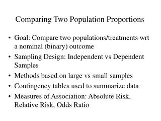
Two-Sample Problems • Comparing two populations or two treatments is one of the most common situations encountered in statistical practice. We call such situations two-sample problems.
Two-Sample Problems • A two-sample problem can arise from a randomized comparative experiment that randomly divides subjects into two groups and exposes each group to a different treatment, like the PROVE-IT Study. • Comparing random samples separately selected from two populations, like the successful and failed small businesses, is also a two-sample problem. • Unlike the matched pairs designs studied earlier, there is no matching of units in the two samples and two samples can be of different sizes. • Inference procedures for two-sample data differ from those of matched pairs.
Comparing Means and Proportions • Who is more likely to binge drink: male or female college students? • This is obviously a two-sample problem because we are comparing the population of male college students to female college students. • To conduct this study, the Harvard School of Public Health surveyed random samples of male and female undergraduates at four-year colleges and universities about their drinking behaviors. • This observational study was designed to compare the proportion of undergraduate males who binge drink with the proportion of undergraduate females who binge drink.
Comparing Means and Proportions • A bank wants to know which of two incentive plans will most increase the use of its credit cards. • We are comparing the effect of two different treatments here, so it is a two-sample problem. • It offers each incentive to a random sample of credit card customers and compares the amount charged during the following six months. • This is a randomized experiment designed to compare the mean amount spent under each of the two incentive “treatments.”
Chapter 13 Section 1 Comparing Two Means HW: 13.1, 13.2, 13.4, 13.6, 13.8, 13.10, 13.11, 13.14, 13.16
Comparing Two Means • We can examine two-sample data graphically by comparing dotplots or stempots (for small samples) and boxplots or histograms (for large samples). • Now we will apply the ideas of formal inference in this setting. • When both population distributions are symmetric, and especially when they are approximately Normal, a comparison of the mean responses in the two populations is the most common goal of inference.
Notation • There are four unknown parameters, the two means and the two standard deviations. • We want to compare the two population means, either by giving a confidence interval for their difference µ1 - µ2 or by testing the hypothesis of no difference, H0:µ1= µ2. • We use the sample means and standard deviations to estimate the unknown parameters.
Calcium and Blood Pressure • Does increasing the amount of calcium in our diet reduce blood pressure? • An examination of a large number of people revealed a relationship between calcium intake and blood pressure. The relationship was strongest for black men. As a result, researchers designed a randomized comparative experiment. • The subjects were 21 healthy black men. A randomly chosen group of 10 of the men received calcium supplements for 12 weeks. The other 11 men received a placebo pill that looked similar for the 12 weeks.
Calcium and Blood Pressure • The response variable is the decrease in systolic blood pressure for a subject after 12 weeks. An increase appears as a negative response. • Group 1 will be the calcium group and Group 2 will be the placebo group. Here are the data. • Here are the summary statistics.
Calcium and Blood Pressure • Notice that the calcium group experienced a drop in blood pressure, while the placebo group shows a small increase, Is this good evidence that calcium decreases blood pressure in the entire population of healthy black men more than a placebo does? • This example fits the two-sample setting because we have a separate sample from each treatment and we have not attempted to match them. • Since we are testing a claim, we will conduct a significance test and follow the Inference Toolbox.
Calcium and Blood Pressure • Step 1: Hypotheses – We write the hypotheses in terms of the mean decreases we would see in the entire population μ1 of black men taking calcium for 12 weeks and μ2 for black men taking the placebo for 12 weeks. There are two possible hypotheses: or
Calcium and Blood Pressure • Step 2 – Conditions – We do not know the name of the test, but we know the conditions we must check to compare two means. • SRS – The 21 subjects are not an SRS. Therefore, we may not be able to generalize our findings to all healthy black men. Since we randomly assigned treatments, however, any differences can be attributed to the treatments themselves. • Normality – Since we have small samples, we must look at a boxplot and histogram for both samples. There are no serious problems (outliers or serious departure from Normality). • Independence – Since we randomized the treatments, we can safely assume that the calcium and placebo are two independent samples.
Calcium and Blood Pressure • The natural estimator of the difference µ1 - µ2 is the difference between the sample means: • This statistic measures the average advantage of calcium over the placebo. In order to use this, however, we need to know about its sampling distribution. In other words, we need to know what the mean and standard deviation would be for the population of differences if we took repeated samples many times.
The Two-Sample z Statistic • Here are the facts about the sampling distribution of the difference between the two sample means of independent SRSs. • Therefore, • If both populations are Normal, then the distribution of is also Normal with
Two-Sample z Statistic • When the statistic has a Normal distribution, we can standardize it to obtain a standard Normal z statistic.
Two-Sample z Statistic • In the very unlikely case that we know both population standard deviations, the two-sample z statistic is what we would use to conduct inference about • Since we rarely know one, much less two, population standard deviations, we are going to move immediately to the more useful t procedures.
Two-Sample t Procedures • Because we don’t know the population standard deviations, we estimate them with the standard deviations from our two samples. • The result is the standard error, or estimated standard deviation, of the difference in sample means: • We then standardize our estimate the result if the two-sample t statistic:
Two-Sample t Procedures • The statistic t has the same interpretation as any z or t statistic: it says how far is from its mean in standard deviation units. • The two-sample t statistic has approximately a t distribution. It does not have exactly a t distribution even if the populations are both exactly Normal. The approximation is very close though. • There is a catch: we must use a messy formula to calculate the degrees of freedom. Often, the degrees of freedom are not whole numbers.
Two-Sample t Procedures • There are two practical options for using the two-sample t procedures: • With technology, use the statistic t with accurate critical values from the approximating t distribution. • Without technology, use the statistic t with critical values from the t distribution with degrees of freedom equal to the smaller of n1 – 1 and n2 – 1. These procedures are always conservative for any two Normal populations. • Technology will obviously use method 1. • We are going to start by looking at how to do method 2.
Two-Sample t Procedures • These two-sample t procedures always err on the safe side, reporting higher P-values and lower confidence than may actually be true. The gap between what is reported and the truth is actually quite small unless the sample sizes are both small and unequal. • As the sample sizes increase, probability values based on t with degrees of freedom equal to the smaller of n1 – 1 and n2 – 1 become more accurate. • Lets complete our calcium and blood pressure problem from earlier.
Calcium and Blood Pressure • Here are the summary statistics again. • Step 3 – Calculations • Since it was a one-sided test, we are looking for the probability being 1.604 or greater when we have 9 degrees of freedom. From the table, it is between 0.05 and 0.10.
Calcium and Blood Pressure • Step 4 – Interpretation • The experiment provides some evidence that calcium reduces blood pressure, but the evidence falls short of the traditional 5% and 1% levels of significance. We would fail to reject H0 at both significance levels.
Creating a Confidence Interval • We can estimate the difference in mean decreases in blood pressure for the hypothetical calcium and placebo populations using a two-sample t interval. • We have already checked all of the conditions. • Recall • Since the 90% confidence interval includes 0, we cannot reject H0:μ1 – μ2 = 0 against the two-sided alternative at the α = 0.10 level of significance.
Sample Size Matters • Sample sizes strongly influence the P-value of a test. • A result that fails to be significant at a specified level α in a small sample may be significant in a larger sample. • For instance, the difference of 5.273 in the mean systolic blood pressures between our two groups was not significant. In a larger study with more subjects, they were able to obtain a P-value of 0.008.
Robustness Again • The two-sample t procedures are more robust than the one-sample t procedures, particularly when the distributions are not symmetric. • When the sizes of the two samples are equal and the two populations being compared have distributions with similar shapes, probability values from the t table are quite accurate for a broad range of distributions for samples as small as 5. When the populations have different shapes, larger samples are needed.
Robustness Again • As a guide to practice, adapt the guidelines on p. 655 for the use of one-sample t procedures to two-sample t procedures by replacing “sample size” with the “sum of the sample sizes” as long as both samples are at least 5. • These guidelines err on the side of safety, especially when the two-samples are of equal size. • Whenever possible, try to make both samples the same size. Two-sample procedures are most robust against non-Normality when the sample sizes are equal and the conservative P-values are most accurate.
Software Approximations for the DF • The t procedures remain exactly as before except that we use the t distribution with df given by the formula in the box above to give critical values and find P-values.
Calcium and Blood Pressure • Here are the summary statistics again. • For improved accuracy, lets calculate the df given by the formula on the prior slide.
Notice that the P-value here is 0.064 compared to the 0.0716 we got from the conservative approach.
Degrees of Freedom • The formula from the box will always give us df at least as large as the smaller of the two samples and never bigger than n1 + n2 -2. • The number of degrees of freedom is generally not a whole number. Since the table only has whole numbers, we will need to use technology to do these calculations easily. • Let’s do the Calcium and Blood Pressure problem on the calculator! • We should use the calculator to do these calculations from now on!
DDT Poisoning • Poisoning by the pesticide DDT causes convulsions in humans and other mammals. Researchers seek to understand how the convulsions are caused. In a randomized comparative experiment, the compared 6 white rats poisoned with DDT with a control group of 6 unpoisoned rats. Electrical measurements of nerve activity are the main clue to the nature of DDT poisoning. When a nerve is stimulated, its electrical response shows a sharp spike followed by a much smaller second spike. The experiment found that the second spike is larger in rats fed DDT than in normal rats.
DDT Poisoning • The researchers measured the height (or amplitude) of the second spike as a percent of the first spike when a nerve in the rats leg was stimulated. • For the poisoned rats the results were: • For the control group the results were: • Let’s conduct a significance test at the 0.05 significance level to determine if there is a difference using the calculator.
DDT Poisoning • Step 1 – Hypotheses • We want to compare the mean height μ1 of the second-spike electrical response in rats fed DDT with the mean height μ2 of the second-spike electrical response in the population of normal rats. Or
DDT Poisoning • Step 2 – Conditions – Since both population standard deviations are unknown we need to conduct a 2-sample t test. • SRS – By randomly assigning the rats to the treatments, we can conclude that differences are a result of the treatment. The researchers are willing to assume that the two samples of rats represent an SRS. • Normality – We don’t know if the populations are Normal and do not have a large enough sample. We must look at a boxplot and histogram. No outliers or heavy skewness. • Independence – Due to the random assignment, the researchers can treat the two groups as independent.
DDT Poisoning • Step 3 – Calculations • Since it is a two-sided hypothesis, we must find the probability that we are less than -2.99 or greater than 2.99. • The degrees of freedom are df = 5.9 and the P-value from t(5.9) distribution is 0.0246. • Step 4 – Conclusion • Since 0.0246 is less than the significance level of 0.05, we reject the null hypothesis and conclude that there is sufficient evidence to conclude that the height of the second-spike electrical response in rats fed DDT differs from that of normal rats.
Pooled Two-Sample t Procedures • Do not use them. • If a printout says pooled, do not use that. Instead use the one that says unpooled. • On the calculator, always do No for pooled. • If you want more information you can read it on p. 800.
Chapter 13 Section 2 Comparing Two Proportions HW: 13.26, 13.27, 13.28, 13.29, 13.30, 13.32, 13.33, 13.38
Prayer and In Vitro Pregnancy • Some women want to have children but cannot for medical reasons. One option for these women is in vitro fertilization. About 28% of women who undergo in vitro fertilization get pregnant. Can praying for these women help increase the pregnancy rate? • Researchers developed an experiment to help answer this question. (Why not just survey women who have already gone through in vitro to find out if a higher percentage of women who were prayed for got pregnant?)
Prayer and In Vitro Pregnancy • A large group of women who were about to undergo in vitro fertilization served as the subjects. Each subject was randomly assigned to the treatment group (prayed for by people who did not know them) or a control group (no prayer). • The results: 44 of the 88 women (50%) got pregnant in the treatment (prayer) group while only 21 out of 81 got pregnant in the control group. • This seems like a large difference, but is it statistically significant?
Two-Sample Proportions • We will use notation that is similar to what we used for two-sample means. We still want to compare two groups, Population 1 and Population 2. • Here is the notation: • We compare the populations by doing inference about the difference p1- p2 between the population proportions. • The statistic that estimates this difference is