IC Manufacturing and Yield
IC Manufacturing and Yield. ECE/ChE 4752: Microelectronics Processing Laboratory. Gary S. May April 15, 2004. Outline. Introduction Statistical Process Control Statistical Experimental Design Yield. Motivation.


IC Manufacturing and Yield
E N D
Presentation Transcript
IC Manufacturing and Yield ECE/ChE 4752: Microelectronics Processing Laboratory Gary S. May April 15, 2004
Outline • Introduction • Statistical Process Control • Statistical Experimental Design • Yield
Motivation • IC manufacturing processes must be stable, repeatable, and of high quality to yield products with acceptable performance. • All persons involved in manufacturing an IC (including operators, engineers, and management) must continuously seek to improve manufacturing process output and reduce variability. • Variability reduction is accomplished by strict process control.
Production Efficiency • Determined by actions both on and off the manufacturing floor • Design for manufacturability (DFM): intended to improve production efficiency
Variability • The most significant challenge in IC production • Types of variability: • human error • equipment failure • material non-uniformity • substrate inhomogeneity • lithography spots
Deformations • Variability leads to => deformations • Types of deformations 1) Geometric: • lateral (across wafer) • vertical (into substrate) • spot defects • crystal defects (vacancies, interstitials) 2) Electrical: • local (per die) • global (per wafer)
Outline • Introduction • Statistical Process Control • Statistical Experimental Design • Yield
Statistical Process Control • SPC = a powerful collection of problem solving tools to achieve process stability and reduce variability • Primary tool = the control chart; developed by Dr. Walter Shewhart of Bell Laboratories in the 1920s.
Control Charts • Quality characteristic measured from a sample versus sample number or time • Control limits typically set at 3s from center line (s = standard deviation)
Control Chart for Attributes • Some quality characteristics cannot be easily represented numerically (e.g., whether or not a wire bond is defective). • In this case, the characteristic is classified as either "conforming" or "non- conforming", and there is no numerical value associated with the quality of the bond. • Quality characteristics of this type are referred to as attributes.
Defect Chart • Also called “c-chart” • Control chart for total number of defects • Assumes that the presence of defects in samples of constant size is modeled by Poisson distribution, in which the probability of a defect occurring is where x is the number of defects and c > 0
Control Limits for C-Chart • C-chart with ± 3s control limits is given by Centerline = c (assuming c is known)
Control Limits for C-Chart • If c is unknown, it can be estimated from the average number of defects in a sample. • In this case, the control chart becomes Centerline =
Example Suppose the inspection of 25 silicon wafers yields 37 defects. Set up a c-chart. Solution: Estimate c using This is the center line. The UCL and LCL can be found as follows Since –2.17 < 0, we set the LCL = 0.
Defect Density Chart • Also called a “u-chart” • Control chart for the average number of defects over a sample size of n products. • If there are c total defects among the n samples, the average number of defects per sample is
U-chart with ± 3s control limits is given by: Center line = where u is the average number of defects over m groups of size n Control Limits for U-Chart
Suppose an IC manufacturer wants to establish a defect density chart. Twenty different samples of size n = 5 wafers are inspected, and a total of 183 defects are found. Set up the u-chart . Solution: Estimate u using This is the center line. The UCL and LCL can be found as follows Example
Control Charts for Variables • In many cases, quality characteristics are expressed as specific numerical measurements. • Example: the thickness of a film. • In these cases, control charts for variables can provide more information regarding manufacturing process performance.
Control of Mean and Variance • Control of the mean is achieved using an -chart: • Variance can be monitored using the s-chart, where:
Control Limits for Mean where the grand average is:
Control Limits for Variance where: and c4 is a constant
Modified Control Limits for Mean • The limits for the -chart can also be written as:
Example Suppose and s-charts are to be established to control linewidth in a lithography process, and 25 samples of size n = 5 are measured. The grand average for the 125 lines is 4.01 mm. If = 0.09 mm, what are the control limits for the charts? Solution: For the -chart:
Example Solution (cont.): For the s-chart:
Outline • Introduction • Statistical Process Control • Statistical Experimental Design • Yield
Background • Experiments allow us to determine the effects of several variables on a given process. • A designed experiment is a test or series of tests which involve purposeful changes to variables to observe the effect of the changes on the process. • Statistical experimental design is an efficient approach for systematically varying these process variables and determining their impact on process quality. • Application of this technique can lead to improved yield, reduced variability, reduced development time, and reduced cost.
Comparing Distributions • Consider the following yield data (in %): • Is Method B better than Method A?
Hypothesis Testing • We test the hypothesis that B is better than A using the null hypothesis: H0: mA = mB • Test statistic: where: are sample means of the yields, ni are number of trials for each sample, and
Results • Calculations: sA = 2.90 and sB = 3.65, sp = 3.30, and t0 = 0.88. • Use Appendix K to determine the probability of computing a given t-statistic with a certain number of degrees of freedom. • We find that the likelihood of computing a t-statistic with nA + nB - 2 = 18 degrees of freedom = 0.88 is 0.195. • This means that there is only an 19.5% chance that the observed difference between the mean yields is due to pure chance. • We can be 80.5% confident that Method B is really superior to Method A.
Analysis of Variance • The previous example shows how to use hypothesis testing to compare 2 distributions. • It’s often important in IC manufacturing to compare several distributions. • We might also be interested in determining which process conditions in particular have a significant impact on process quality. • Analysis of variance (ANOVA) is a powerful technique for accomplishing these objectives.
ANOVA Example • Defect densities (cm-2) for 4 process recipes: • k = 4 treatments • n1 = 4, n2 = n3 = 6, n4 = 8; N = 24 • Treatment means: • Grand average:
Sums of Squares • Within treatments: • Between treatments: • Total:
Within treatments: Between treatments: Total: Degrees of Freedom
Within treatments: Between treatments: Total: Mean Squares
Conclusions • If null hypothesis were true, sT2/sR2 would follow the F distribution with nT and nR degrees of freedom. • From Appendix L, the significance level for the F-ratio of 13.6 with 3 and 30 degrees of freedom is 0.000046. • This means that there is only a 0.0046% chance that the means are equal. • In other words, we can be 99.9954% sure that real differences exist among the four different processes in our example.
Factorial Designs • Experimental design: organized method of conducting experiments to extract maximum information from limited experiments • Goal: systematically explore effects of input variables, or factors (such as processing temperature), on responses (such as yield) • All factors varied simultaneously, as opposed to "one-variable-at-a-time“ • Factorial designs: consist of a fixed number of levels for each of a number of factors and experiments at all possible combinations of the levels.
2-Level Factorials • Ranges of factors discretized into minimum, maximum and "center" levels. • In 2-level factorial, minimum and maximum levels are used together in every possible combination. • A full 2-level factorial with n factors requires 2n runs. • Combinations of a 3-factor experiment can be represented as the vertices of a cube.
23 Factorial CVD Experiment • Factors: temperature (T), pressure (P), flow rate (F) • Response: deposition rate (D)
Main Effects • Effect of any single variable on the response • Computation method: find difference between average deposition rate when pressure is high and average rate when pressure is low: P = dp+ - dp- = 1/4[(d2 + d4 + d6 + d8) - (d1 + d3 + d5 + d7)] = 40.86 where P = pressure effect, dp+ = average dep rate when pressure is high, dp- = average rate when pressure is low • Interpretation: average effect of increasing pressure from lowest to highest level increases dep rate by 40.86 Å/min. • Other main effects for temperature and flow rate computed in a similar manner • In general: main effect = y+ - y-
Interaction Effects • Example: pressure by temperature interaction (P × T). • This is ½ difference in the average temperature effects at the two levels of pressure: P × T = dPT+ - dPT- = 1/4[(d1 + d4 + d5 + d8) - (d2 + d3 + d6 + d7)] = 6.89 • P × F and T × F interactions are obtained similarly. • Interaction of all three factors (P × T × F): average difference between any two-factor interaction at the high and low levels of the third factor: P × T × F = dPTF+ - dPTF- = -5.88
Yates Algorithm • Can be tedious to calculate effects and interactions for factorial experiments using the previous method described above, • Yates Algorithm provides a quicker method of computation that is relatively easy to program • Although the Yates algorithm is relatively straightforward, modern analysis of statistical experiments is done by commercially available statistical software packages. • A few of the more common packages: RS/1, SAS, and Minitab
Yates Procedure • Design matrix arranged in standard order (1st column has alternating - and + signs, 2nd column has successive pairs of - and + signs, 3rd column has four - signs followed by four + signs, etc.) • Column y contains the response for each run. • 1st four entries in column (1) obtained by adding pairs together, and next four obtained by subtracting top number from the bottom number of each pair. • Column (2) obtained from column (1) in the same way • Column (3) obtained from column (2) • To get the Effects, divide the column (3) entries by the Divisor • 1st element in Identification (ID) column is grand average of all observations, and remaining identifications are derived by locating the plus signs in the design matrix.
Fractional Factorial Designs • A disadvantage of 2-level factorials is that the number of experimental runs increasing exponentially with the number of factors. • Fractional factorial designs are constructed to eliminate some of the runs needed in a full factorial design. • For example, a half fractional design with n factors requires only 2n-1 runs. • The trade-off is that some higher order effects or interactions may not be estimable.
Fractional Factorial Example • 23-1 fractional factorial design for CVD experiment: • New design generated by writing full 22 design for P and T, then multiplying those columns to obtain F. • Drawback: since we used PT to define F, can’t distinguish between the P × T interaction and the F main effect. • The two effects are confounded.
Outline • Introduction • Statistical Process Control • Statistical Experimental Design • Yield
Definitions • Yield: percentage of devices or circuits that meet a nominal performance specification. • Yield can be categorized as functional or parametric. • Functional yield - also referred to as "hard yield”; characterized by open or short circuits caused by defects (such as particles). • Parametric yield – proportion of functional product that fails to meet performance specifications for one or more parameters (such as speed, noise level, or power consumption); also called "soft yield"
Functional Yield Y = f(Ac, D0) Ac = critical area (area where a defect has high probability of causing a fault) D0 = defect density (# defects/unit area)
Poisson Model • Let: C = # of chips on a wafer, M = # of defect types • CM = number of unique ways in which M defects can be distributed on C chips • Example: If there are 3 chips and 3 defect types (such as metal open, metal short, and metal 1 to metal 2 short, for example), then there are: CM = 33 = 27 possible ways in which these 3 defects can be distributed over 3 chips