Exploring Black Box Methods in Linear Elastostatics: Green's Functions and Fast Algorithms

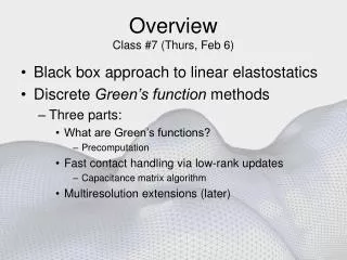
1. OverviewClass #7 (Thurs, Feb 6) • Black box approach to linear elastostatics • Discrete Green’s function methods • Three parts: • What are Green’s functions? • Precomputation • Fast contact handling via low-rank updates • Capacitance matrix algorithm • Multiresolution extensions (later)

2. Small-strain time-independent (static/equilibrium) deformation response Various origins, e.g., solid bodies, thin shells, abstract linear systems, … Various surface representations and discretization possible, e.g., FEM, BEM, FVM, FDM, spectral,… Linear Elastostatic Models (recap from last class)

3. GF Deformation Basis • Green’s functions are physically based basis functions adapted to • particular geometry • particular constraints • GF matrix is an input-output model of the linear deformable system (for a particular BVP-type) • Relates displacements to tractions, etc. • We’ll focus on surface constraints & surface GFs • Also works for volumetric quantities • displacement, stress, strain, strain-rate, etc.

4. Some Graphics References • See webpage • Cotin et al., 96/99. • James & Pai • ARTDEFO: Accurate Real Time Deformable Objects, In SIGGRAPH 99 Conference Proceedings, ACM SIGGRAPH, 1999. • A Unified Treatment of Elastostatic and Rigid Contact for Real Time Haptics, Haptics-e, The Electronic Journal of Haptics Research (www.haptics-e.org), 2(1), 2001. • Doug L. James and Dinesh K. Pai, Multiresolution Green's Function Methods for Interactive Simulation of Large-scale Elastostatic Objects, ACM Transactions on Graphics, Volume 22, No. 1, Jan. 2003. • …

5. Discrete Green's Functions (GFs)(in a nutshell...) • Reference BVP (RBVP) • Green’s function matrix • General solution to RBVP (barspecified BV)

6. Example: Displacement Constrained Model (white dots indicate “fixed” vertices)

7. Corresponding Green’s Functions • GF for this vertex is the response due to a vertex force in the x, y and z directions • Use linear superposition to combine responses

8. Block influence coefficient describes effect of jth SBV on ith UBV. Anatomy of a Green’s Function • GF column corresponding to jth node, j

9. Anatomy of a Green’s Function • GF corresponding to a single vertex…

10. Boundary Value Notation • Various model descriptions/spaces possible • Variables defined at n nodes/vertices: x=(x1,x2,…,xn)T • Continuous displacement u(x) and traction p(x) fields, e.g., • Discrete displacement u and traction p fields, e.g., u=(u1,u2,…,un)T, uk=u(xk) p=(p1,p2,…,pn)T, pk=p(xk) • Force relationship: fk=akpk, ak=kd • Sign convention: (uk,pk)0

11. Boundary Value Problem (BVP) • Specified and unspecified nodal variables • (u, p) are complementary node sets specifying nodes with u or p constraints • BVP: Given and (u, p) Compute v • (Mixed nodal boundary conditions possible)

12. Example: BEM (from last class) Identification with BEM equations Hu=Gp (ARTDEFO paper)

13. Specify boundary conditions Red: BV specified Yellow: BV unknown Recap: Solving the BVP •  A v = z, A large, dense H u = G p H,G large & dense

14. Green's Functions (GFs) • Reference BVP (RBVP) • Green’s function matrix • Solutions to RBVP are

15. Data-driven GF Formulation • Excellent for interactive applications! • Precompute GFs for speed • Exploits linearity • Avoids redundant work • Optional boundary-only description for speed • “Black-box” model definition

16. Force-feedback Rendering

17. More generally... • GFs: fundamental response of a linear system • See whiteboard: • If Lu=f + BVP then GF, G, satisfies LG=delta + homog BC. • In linear elasticity, there are formulae for “free space” solutions, and a few others. • Survey of GFs for other physical phenomena • We want Green’s functions for a particular deformable object (& constraint configuration), hence • Numerical approx  “discrete Green’s functions”

18. Fast Capacitance Matrix Algorithms ARTDEFO: Accurate Real Time Deformable Objects In SIGGRAPH 99 Conference Proceedings, ACM SIGGRAPH, 1999. (with Dinesh K. Pai) A Unified Treatment of Elastostatic and Rigid Contact for Real Time Haptics, Haptics-e, The Electronic Journal of Haptics Research (www.haptics-e.org), 2(1), 2001. (w/ DKP)

19. A(0)v(0)=z(0) A(1)v(1)=z(1) A(2)v(2)=z(2) A(3)v(3)=z(3) Exploiting BVP Equation Structure

20. Boundary Value Changes Constraint type (positionforce) doesn’t change Only the value of the constraint changes

21. = H u = G p A v = z Boundary Value Changes • BV changes only affect z in Av=z • Traction-free BC are trivial: • 0+0+0+...

22. Boundary Condition Type Changes Position  Force constraint type switching Intermediate BV changes

23. = H u = G p = + A v = z Boundary Condition Type Changes • BC change swaps a block column of A

24. If = Sherman-Morrison-Woodbury • Idea: Exploit coherence between BVPs • s-by-s capacitance matrix • Smaller matrix to invert and store!

25. Motivation: Changing BVP Type • Tractiondisplacement constraint switching • Example: single nonzero constraint:  Self-effect relationship:  Equivalent traction constraint:  Equivalent Green’s function (displ. constraint): • Systematic formulation is CMA

26. Capacitance Matrix Algorithms • Solving general BVP using RBVP’s GFs • Low-rank updating techniques • Long history in computing: • Sherman-Morrison-Woodbury et al. (`50) • Static reanalysis • Contact mechanics [Ezawa & Okamoto 89] • Domain decomposition • Real time simulation with precomputed GF [Cotin et al. 96, JamesPai99]

27. CMA: Notation • Updated capacitance node list, S S=(S1,S2,…,Ss) for s updates. • Contact compliance matrix, C • C = -ETE • Capacitance matrix • E: densesparse row expansion • e.g., S={k}, E=I:k3n3 • ET: sparsedense row extraction

28. CMA: Formulae • Solution to any BVP in terms of  • Direct solver with input/output sensitivity • O(s3) C-1 construction for s switched contacts • O(s2+sn) solve for s nonzero BC and n outputs • Using Sherman-Morrison-Woodbury... • v = v(0) + (E+(E)) C-1ET v(0) • v(0) = [ (I-EET) - EET ] v + B • C = -ETE = s-by-scapacitance matrix _

29. CMA: Formulae (cont’d)

30. v = v(0) + (E+(E)) C-1ET v(0) • v(0) = [ (I-EET) - EET ] v + B • C = -ETE = s-by-scapacitance matrix Capacitance Matrix Algorithm (CMA) • Compute C-1 • Compute v(0) • Compute s updated BVs: ET v = C-1ET v(0) 3s • Add correction to v(0) to obtain v: v(0) += (E+(E)) (C-1ET v(0)) (Simpler when v(0) = -v ) _ _

31. Demo!

32. Early ARTDEFO Examples ARTDEFO: Accurate Real Time Deformable Objects In SIGGRAPH 99 Conference Proceedings, ACM SIGGRAPH, 1999. (with Dinesh K. Pai)

33. Capacitance Inverse Updating • Sequential inversion • Use one C-1 to construct another • Exploits temporal coherence between matrix BVP • O(s2s) cost for s BC changes • Effective updating of explicit matrix inverse

34. Capacitance Inverse Updating

35. Haptic Interaction