Download
1 / 18
180 likes | 284 Vues
Explore the final results and conclusions of drift cell simulation, along with the methods and tools used for parametrization in this study by A. Gresele & T. Rovelli from Bologna University & INFN.

E N D
1 Final Results of Drift CellSimulation and Parametrization • A. Gresele and T. Rovelli • Bologna University & INFN • Cell Simulation Procedure • Method Used to Parametrize • Final Results • Conclusions A. Gresele - CMS week
2 Simulated Tracks Granularity • 1 mm between x = 0 cm and 2 cm; • 5 degree between d = 0o and 45o (between d = -45o and 45o when Bw not 0) • 0.03 T between Bd = 0 and 0.3 T • 0.1 T between Bn = 0 and 1 T • 0.03 T between Bw = 0 • and 0.3 T Bn Bw Bd Only BnBw and BnBd pairs to reduce the num- ber of simulated tracks. x sense wire cathode track A. Gresele - CMS week
3 Method Used to Producethe Drift Times • Full simulation on ALPHA machines ; • Bologna Condor facility used ; • Four tracks for each x, , B considered . • • For each track we assumed the drift time is given by : • 50% one electron • 40% two electrons • 10% three electrons A. Gresele - CMS week
4 Method Used to Parametrizethe Drift Times • The drift lines are more complicated when there is a magnetic field component along the sense wire , Bw . • we used different methods for the parametrization with Bw and Bn. A. Gresele - CMS week
5 • Drift Lines • when • Bw = 0.3 T A. Gresele - CMS week
6 Drift Time Variations with the track angle when B = 0 • To study the dependence of the drift time on the track, we calculated the difference between the drift time with 0 o and = 0 o . • This variation is given in function of the track angle for 3 points , x = 0.6cm, x= 1.1cm and x = 1.6cm. • xpos = 0.6 cm • xpos = 1.1 cm • xpos = 1.6 cm A. Gresele - CMS week
7 Parametrization of Drift Times vs Bw • We performs the regressions on the data for each , x and Bw with HPARAM • (in PAW). • This in order to find the best polinomial parametrization of the drift time. A. Gresele - CMS week
8 To study the quality of the fit we plot the difference between the parametrization and the points. These differences are 6ns. A. Gresele - CMS week
9 Parametrization of Drift Timeswhen Bn 0 xpos = 1.7 cm Bn = 1 T - Bn = 0 T • The time variation (t) due to Bn is essentially independent of the track angle up to 45o and is fitted with a constant(at fixed position). A. Gresele - CMS week
10 Final Parametrization of Bn • For each value of Bn the results of the fit were plotted as a function of the distance from the wire. • These points were then fitted with a straight line to obtain the final parametrization . • Bn=1.0T-Bn=0T • Bn=0.5T-Bn=0T • Bn=0.1T-Bn=0T A. Gresele - CMS week
11 Parametrization of Drift Timeswhen Bd 0 • The same procedure was used for Bd. • The deviations are very small and no correction is required. • Bd=0.30T-Bd=0T • Bd=0.15T-Bd=0T • Bd=0.03T-Bd=0T A. Gresele - CMS week
12 Using this method we obtain... total of: • 19 functions to parametrize Bw • 10 functions to take into account Bn A. Gresele - CMS week
13 Checks on parametrization • To check this procedure we generated 50 tracks at 3 points in the cell (x=0.2/0.4/0.6cm) where the expected deviations are largest.The angles and the magnetic field components ( Bn-Bw and Bn-Bd) were chosen randomly. • The differences between the generated drift times and those computed with the parametrization procedure are ,for Bn-Bw, within 8ns and ,for Bn-Bd ,within 6ns. A. Gresele - CMS week
14 and Bd , Bn components are chosen randomly. Bw = 0 T Bn-Bd 0 T A. Gresele - CMS week
15 and Bd , Bw components are chosen randomly Bd = 0 T Bn-Bw 0 T A. Gresele - CMS week
16 -30o < < +30o t 5ns Bw = 0 T Bn-Bd 0 T A. Gresele - CMS week
17 -30o < +30o t 5ns Bd = 0 T Bn-Bw 0 T A. Gresele - CMS week
18 Conclusions • The parametrization procedure looks reasonable. In fact the differences between simulated and parametrized times are less than 8ns ( less than 5 ns if 30o 30o ) ; • This parametrization is going to be introduced into CMSIM. A. Gresele - CMS week