Data Acquisition and Processing

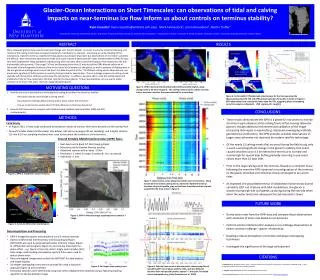
1. Glacier-Ocean Interactions on Short Timescales: can observations of tidal and calving impacts on near-terminus ice flow inform us about controls on terminus stability?Ryan Cassotto1 (ryan.cassotto@wildcats.unh.edu) , Mark Fahnestock2, Jason Amundson3, Martin Truffer2 1Institute for the Study of the Earth, Oceans and Space, University of New Hampshire, Durham, New Hampshire; 2Geophysical Institute, University of Alaska Fairbanks, Fairbanks, Alaska; 3University of Alaska Southeast, Juneau, Alaska ABSTRACT RESULTS Many tidewater glaciers have experienced rapid change over the last decade. Increases in velocity, enhanced thinning, and retreat of the calving fronts have increased Greenland’s contribution to sea level. Improving our understanding of the mechanisms related to terminus stability for these glaciers would seem important, but observations of short-term variability are difficult. Here we present observations made with a pair of ground based portable radar interferometers (GPRI) during a two-week deployment along Jakobshavn Isbrae during which we were able to observe the glacier flow response to the tide and multiple calving events. The range (~16 km) and fast acquisition time (3 minutes) of the GPRI allowed collection of thousands of interferograms showing ice flow in the lower 10+ kilometers of the glacier, as well as patterns of displacement in the pro-glacial ice mélange which covers the fjord. Our data show that of the ~12 different calving events observed only one produced a significant (~33%) increase in velocity that persisted for several days. The ice mélange response to calving varied spatially with the location of those events along the calving face. In addition, we were able to map the spatial extent and amplitude of the ice flow response to the tidal cycle for the lower glacier. These measurements are one way to probe controls on ice flow in the lower reach of a large tidewater glacier. Good agreement 25-Jul-2012 Strain margins not observed by TSX Improvement needed MOTIVATING QUESTIONS Figure 5: GPRI-II derived LOS velocities before (left) and after (right) a large calving event at 23:10 on August 2. The calving event caused a sudden increase in near-terminus velocities that was sustained for several days. How do short-term perturbations at the glacier’s calving front affect the terminus stability - How does velocity vary through a calving event? - How does the mélange affect velocity and/or strain rate at the terminus? - Can we constrain the spatial extent of tidal influence on terminus dynamics? How do GPRI observations compare with satellite based Synthetic Aperture Radar (SAR) and GPS measurements? Figure 6: (L) TerraSAR-X (TSX) derived velocity maps for the time spanning the observation period; (R) TSX and GPRI derived velocities for profile 1 shown in Figure 2. GPRI observations are consistently lower than the TSX, suggesting phase unwrapping correction requires refinement. (TSX courtesy of I. Joughin) North Terminus CONCLUSIONS South Terminus METHODS • These results demonstrate the GPRI is a powerful instrument to monitor short-term perturbations at the calving fronts of fast moving tidewater glaciers; though additional refinement and validation of the image processing techniques is required (e.g. improved unwrapping methods, georeference verification), the GPRI provides valuable observations of target areas otherwise not observed by modern satellite technology. • Of the nearly 12 calving events that occurred during the field study, only 1 event caused significant change in the glacier’s stability; that event caused velocities up to 4.5 km behind the terminus to increase and remain high for several days before gradually returning to pre-event values more than 10 days later. • Prior to the large calving event the terminus flowed as a coherent mass; following the event the GPRI observed a reconfiguration of the terminus as the glacier stretched and velocities slowly converged to pre-event rates. • As expected, the grounded terminus of Jakobshavn Isbrae shows diurnal variability 180° out of phase with tidal modulations, the glacier is slowest during high tide and speeds up during during the low tide when when the water level (and subsequent forced imposed) is lower. • Field Study • In August 2012, 14-day study conducted at Jakobshavn Isbrae to monitor short-term dynamics at the calving front • Ground Portable Radar Interferometer (see below), tide pressure gauges (30-sec sampling), and 3 digital cameras (15-min & 10-sec sampling windows) were used to document the conditions at the terminus. GPRI • Ground Portable RADAR Interferometer (GPRI) Specs • Real Aperture Ku Band (17 GHz) Imaging Radar • Manufactured by Gamma Remote Sensing • Rotational scanner with a radius ~16 km • Resolution: 1-meter in range, 8 meters @ 1 km in azimuth • Sensitivity ~1 mm Profile 2 Profile 1 Figure 1: GPRI at Jakobshavn Isbrae terminus cameras Figure 7: Velocity time-series along two profiles near the terminus. Black horizontal lines denote calving events, diamonds represent terminus locations along each profile, gray vertical lines show the location of pixels sampled for the time-series in figure 8. North Branch 25-Jul-2012 FUTURE WORK Ice Mélange 16-Aug-2012 August 4, 2012 5-Aug-2012 • Derive strain rates from the GPRI data and compare those observations with estimates of strain rate based on ice dynamics. • Perform similar interferometric analysis on ice mélange observations to better constrain mélange – glacier relationships • Develop a robust atmospheric correction and phase unwrapping techniques • Investigate the significance of the large calving event Figure 2: GPRI-II Intensity Image superimposed on Landsat 7 image. South Branch Profile 2 π Figure 3: 3-minute differential interferogram • Data Acquisition and Processing • GPRI-II imaged the glacier and peripheral ice at 3-minute intervals • Gamma’s Differential Interferometry and Geocoding Software (DIFF/GEO) was used to generate backscatter intensity images (figure 2), differential interferograms (figure 3), and unwrap (calculate true phase offset – e.g. figure 5) from the radar’s Single Look Complex (SLC) data; Image multi-looking and adaptive spectral filters were used to reduce phase noise. • Once unwrapped, images were pulled into MATLAB® for data analysis and image displays • 2π integer unwrapping errors were accounted for using a statistical approach (figure 4) and corrected. Stretching Coherent flow Profile 1 -π CITATIONS R. Pawlowicz, B. Beardsley, and S. Lentz, "Classical tidal harmonic analysis including error estimates in MATLAB using T_TIDE", Computers and Geosciences 28 (2002), 929-937. I. Joughin, NASA MEaSURES, DLR for TerraSAR-X derived velocities U.S. Geological Survey. Landsat Images. Department of the Interior/USGS. http://glovis.usgs.gov Figure 8: Velocity time-series at discrete points show strong diurnal variability 180° out of phase with the tides, and also different behavior from two parallel profiles spaced ~ 1 km apart. Predicted record estimated using t-tide (Pawlowicz et al., 2002) Figure 4: 2π integer unwrapping errors • Horizontal velocities were determined using true vector displacements obtained using a featuring tracking algorithm to the backscatter images.