Tutorial: Time-dependent density-functional theory
Tutorial: Time-dependent density-functional theory. Carsten A. Ullrich University of Missouri. XXXVI National Meeting on Condensed Matter Physics Aguas de Lindoia , SP, Brazil May 13, 2013. Outline. PART I: ● The many-body problem ● Review of static DFT PART II:

Tutorial: Time-dependent density-functional theory
E N D
Presentation Transcript
Tutorial: Time-dependent density-functional theory CarstenA. Ullrich University of Missouri XXXVI National Meeting on Condensed Matter Physics Aguas de Lindoia, SP, Brazil May 13, 2013
Outline PART I: ● The many-body problem ● Review of static DFT PART II: ● Formal framework of TDDFT ● Time-dependent Kohn-Sham formalism PART III: ● TDDFT in the linear-response regime ● Calculation of excitation energies
Time-dependent Schrödinger equation kinetic energy operator: electron interaction: The TDSE describes the time evolution of a many-body state starting from an initial state under the influence of an external time-dependent potential
Real-time electron dynamics: first scenario Start from nonequilibrium initial state, evolve in static potential: t=0 t>0 Charge-density oscillations in metallic clusters or nanoparticles (plasmonics) New J. Chem. 30, 1121 (2006) Nature Mat. Vol. 2 No. 4 (2003)
Real-time electron dynamics: second scenario Start from ground state, evolve in time-dependent driving field: t=0 t>0 Nonlinear response and ionization of atoms and molecules in strong laser fields
Coupled electron-nuclear dynamics ● Dissociation of molecules (laser or collision induced) ● Coulomb explosion of clusters ● Chemical reactions High-energy proton hitting ethene T. Burnus, M.A.L. Marques, E.K.U. Gross, Phys. Rev. A 71, 010501(R) (2005) Nuclear dynamics treated classically
Density and current density Heisenberg equation of motion for the density: Similar equation of motion for the current density (we need it later):
The Runge-Gross Theorem (1984) The time evolution and dynamics of a system is determined by the time-dependent external potential, via the TDSE. The TDSE formally defines a map from potentials to densities: fixed To construct a time-dependent DFT, we need to show that the dynamics of the system is completely determined by the time-dependent density. We need to prove the correspondence unique 1:1 for a given
Proof of the Runge-Gross Theorem (I) Consider two systems of Ninteracting electrons, both starting in the same ground state , but evolving under different potentials: The two potential differ by more than just a time-dependent constant. The two different potentials can never give the same density! What happens for potentials differing only by c(t)? They give same density!
Proof of the Runge-Gross Theorem (II) We assume that the potentials can be expanded in a Taylor series about the initial time: Two different potentials: there exists a smallest k so that Step 1: show that the current densities must be different! We start from the equation of motion for the current density. If the two potentials are different at the initial time, then the two current densities will be different infinitesimally later than t0
Proof of the Runge-Gross Theorem (III) If the potentials are not different at the initial time, they will become different later. This shows up in higher terms in the Taylor expansion. Use the equation of motion k times: This proves the first step of the Runge-Gross theorem: unique 1:1 for a given Step 2: show that if the current densities are different, then the densities must be different as well!
Proof of the Runge-Gross Theorem (IV) Calculate the (k+1)st time derivative of the continuity equation: = 0 We must show that right-hand side cannot vanish identically! Use Green’s integral theorem: positive, cannot vanish = 0 so, this term cannot vanish! Therefore, the densities must be different infinitesimally after t0. This completes the proof.
The Runge-Gross Theorem E. Runge and E.K.U. Gross, Phys. Rev. Lett. 52, 997 (1984) The potential can therefore be written as a functional of the density and initial state, which determines the Hamiltonian: All physical observables become functionals of the density: unique 1:1 for a given
The van Leeuwen Theorem In practice, we want to work with a noninteracting (Kohn-Sham) system that reproduces the density of the interacting system. But how do we know that such a noninteracting system exists? (this is called the “noninteracting V-representability problem”) R. van Leeuwen, Phys. Rev. Lett. 82, 3863 (1999) ● Can find a system with a different interaction that reproduces the same density. In particular, w=0 is a noninteracting system. ● This provides formal justification of the Kohn-Sham approach ● Proof requires densities and potentials to be analytic at initial time. Recently, examples of nonanalytic densities were discovered: Z.-H. Yang, N.T. Maitra, and K. Burke, Phys. Rev. Lett. 108, 063003 (2012)
1 ● TDDFT works for periodic systems if the time-dependent potential is also periodic in space. ● The RG theorem does not apply when a homogeneous electric field (a linear potential) acts on a periodic system. Solution: upgrade to time-dependent current-DFT 2 N.T. Maitra, I. Souza, and K. Burke,PRB68, 045109 (2003) Situations not covered by the RG theorem TDDFT does not apply for time-dependent magnetic fields or for electromagnetic waves. These require vector potentials. The original RG proof is for finite systems with potentials that vanish at infinity (step 2). Extended/periodic systems can be tricky:
Time-dependent Kohn-Sham scheme (I) Consider anN-electron system, starting from a stationary state. Solve a set of static KS equations to get a set of N ground-state orbitals: The N static KS orbitals are taken as initial orbitals and will be propagated in time: Time-dependent density:
Dependence on densities: (nonlocal in space and time) The time-dependent xc potental Dependence on initial states, except when starting from the ground state Static DFT: TDDFT: more complicated! (stationary action principle)
Time-dependent self-consistency Time propagation requires keeping the density at previous times stored in memory! (But this is almost never done in practice….)
depends on density at time t (instantaneous, no memory) Adiabatic approximation is a functional of Adiabatic approximation: (Take xc functional from static DFT and evaluate with the instantaneous time-dependent density) ALDA:
Numerical time propagation Propagate a time step Crank-Nicholson algorithm: Problem: must be evaluated at the mid point But we know the density only for times use “predictor-corrector scheme”
1 2 3 Summary of TDKS scheme: 3 steps Prepare the initial state, usually the ground state, by a static DFT calculation. This gives the initial orbitals: Solve TDKS equations selfconsistently, using an approximate time-dependent xc potential which matches the static one used in step 1. This gives the TDKS orbitals: Calculate the relevant observable(s) as a functional of
Observables: the time-dependent density The simplest observable is the time-dependent density itself: Electron density map of the myoglobin molecules, obtained using time-resolved X-ray scattering. A short-lived CO group appears during the photolysis process. Schotte et al., Science 300, 1944 (2003)
Observables: the particle number Unitary time propagation: During an ionization process, charge moves away from the system. Numerically, we can describe this on a finite grid with an absorbing boundary. The number of bound/escaped particles at time t is approximately given by
Observables: moments of the density dipole moment: sometimes one wants higher moments, e.g. quadrupole moment: One can calculate the Fourier transform of the dipole moment: Dipole power spectrum:
Example: Na9+ cluster in a strong laser pulse off resonance on resonance a lot of ionization not much ionization Intensity: I=1011 W/cm2
Implicit density functionals We have learned that in TDDFT all quantum mechanical observables become density functionals: Some observables (e.g., the dipole moment), can easily be expressed as density functionals. But there are also difficult cases! ► Probability to find the system in a k-fold ionized state Projector on eigenstates with k electrons in the continuum
Implicit density functionals ►Photoelectron kinetic-energy spectrum ►State-to-state transition amplitude (S-matrix) All of the above observables are easy to express in terms of the wave function, but very difficult to write down as explicit density functionals. Not knowing any better, people often calculate them approximately using the KS Slater determinant instead of the exact wave function. This is an uncontrolled approximation, and should only be done with great care.
Ionization of a Na9+ cluster in a strong laser pulse 25 fs laser pulses 0.87 eV photon energy I=4x10¹³ W/cm2 For implicit observables such as ion probabilities one needs to make two approximations: for the xc potential in the TDKS calculation (2) for calculating the observable from the TDKS orbitals.
CO2 molecule in a strong laser pulse (a 30 Mb movie of the time-dependent density of the molecule goes here) Calculation done with octopus