Download
1 / 41
430 likes | 594 Vues
Choice of Mode. David Levinson. The Onion. A study by the American Public Transportation Association reveals that 98 percent of Americans support the use of mass transit by others.” They reported on a campaign supposedly kicked off by APTA "Take The Bus... I'll Be Glad You Did.".

E N D
Choice of Mode David Levinson
The Onion • A study by the American Public Transportation Association reveals that 98 percent of Americans support the use of mass transit by others.” They reported on a campaign supposedly kicked off by APTA "Take The Bus... I'll Be Glad You Did."
Richardson Arms Race Model • Lewis Frye Richardson, a Quaker physicist, suggested that an arms race can be understood as an interaction between two states with three motives. • Grievances between states cause them to acquire arms to use against one another. • States fear each other and so acquire arms to defend themselves against the others’ weapons. • Because weapons are costly, their expense creates fatigue that decreases future purchases.
Example • ArmsRace.xls
How Does This Relate To Transport/Land Use • Arms Races • Bicycle vs. Car • Bus vs. Car • SUV vs. Car • Communities fighting for development, • Communities building infrastructure (competitive advantage/disadvantage)
Caveat Planner • Richardson’s (or any abstract) model is obviously a simplification. We can relax assumptions and make it more realistic (e.g. (dis)economies of scale associated with arms … does fatigue per unit of armament increase or decrease with total level of armaments?)
Repeated Prisoner’s Dilemma • If 2 players, and game repeated indefinitely, the incentive is to cooperate. • However if the end is known, the incentive is to defect on the previous turn. • Also, if there are multiple players, cooperation becomes much more difficult to achieve
Model 1 • Here we assumed the following: • MA = Auto Mode Share • MB = Bus Mode Share = 1 – Auto Mode Share • TA= Auto Travel Time • TB = Bus Travel Time
Model 2 • D = Schedule Delay
Implications • Driving is always faster than riding the bus. • Total travel time would be minimized if everyone rode the bus. Buses could operated frequently and more directly. • However, in the absence of cooperation, the rational outcome is for everyone to drive. • Cooperation is difficult to achieve in multi-player games.
Cooperation • How can cooperation be achieved?
Individual Rationality • Assumption: Individuals will do what is in their own long term interest. • This can’t always be measured. • Max U = f( time, money, socioeconomics, demographics, etc.)
Objective of Mode Choice • AGGREGATE: Estimate the number of trips from each zone to each zone by purpose that take mode m. • DISAGGREGATE: Estimate the probability that a particular trip (purpose, time, zone-zone) by a specific individual will take mode m. • Typically forecasters use a “discrete choice” model, that predicts distinct (or discrete or qualitative) choices (bus vs. car) rather than continuous ones (3.4 trips vs. 3.6). • Logit is the most popular version of mode choice model.
Daniel McFadden • In addition to being my Econometrics Professor in grad school, University of Minnesota graduate Daniel McFadden won the Nobel Prize in Economics for developing the Logit model for transportation mode choice • In particular, his application of Logit to forecasting for the BART rail system in the San Francisco Bay Area) was noted. • Urban Travel Demand: A Behavioral Analysis by Tom Domencich and Daniel L. McFadden North-Holland Publishing Co., 1975. Reprinted 1996. • http://emlab.berkeley.edu/users/mcfadden/travel.html
Pm - probability of taking mode m Umij- Utility of mode m between OD pair ij for an individual (or a representative traveler) Umij = f(Cij,…) The Logit Model
What Affects Choice of Mode? • Travel Time of trip • Travel time to access mode • Wait Time f(headways of transit vehicles) • Transfer Time • Fare • Parking Costs • Tolls • Alternative Specific Constant • Other Qualitative Data (Sidewalks, Bus Shelters)
Relationship of Logit and Gravity • The functional relationship between the modern gravity model (negative exponential form) and the logit mode choice model are very similar, enabling simultaneous choice models to be easily developed. • The key difference is that the gravity model is typically much more aggregate.
Alternative Structures include Nests Advantages: Nests Allow Model to Capture Relationships between modes, skirt IIA property. Disadvantages: Increased computation, Marginal Improvement in Estimation (WCT) walk connected transit (ADT) auto connect transit (driver alone/park and ride) (APT) auto connect transit (auto passenger/kiss and ride) (AU1) auto driver (no passenger) (AU2) auto 2 occupants (AU3+) auto 3+ occupants (WK/BK) walk/bike Typical Model Structure
Independence of Irrelevant Alternatives • Property of Logit (but not all Discrete Choice models) • If you add a mode, it will draw from present modes in proportion to their existing shares. • Example: Suppose a mode were removed. Where would those travelers go. IIA says they will go to other modes in same proportion that other travelers are currently using them. However, if we eliminated Kiss and Ride, a disproportionate number may use Park and Ride or carpool. Nesting allows us to reduce this problem. However, there is an issue of the proper Nest. • Other alternatives include more complex models (e.g. Mixed Logit) which are more difficult to estimate.
Conclusions • Mode share must be understood as a system involving competition. • This competition, under certain circumstances (without subsidies for positive feedback industries, and without penalties for negative externalities), may result in socially sub-optimal results. • The degree to which the results are sub-optimal, and subsidies are justified, depends on (1) belief that government can actually figure out where to direct subsidy (the pork problem), (2) understanding the dynamics of the system under question. • Not all subsidies are warranted, though many are justfied wrongly based on this logic.
Example • You are given this mode choice model • U=-0.412 (c/w) -0.0201* t - 0.0531*t0 -0.89*D1 - 1.78 D3 - 2.15 D4. • Where: • c/w = cost of mode (cents) / wage rate (in cents per minute) • t = travel time in-vehicle (min) • t0 = travel time out-of-vehicle (min) • D = mode specific dummies: • D1 = driving, • D2 = bus with walk access, [base mode] • D3 = bus with auto access, • D4 = carpool
Solve for Probabilities of Modes • ModeChoice.xls
Problem a • You are given the following mode choice model. • Uij = -1 Cijm + 5 DT • Where: • Cijm = travel time between i and j by mode m • DT = dummy variable (alternative specific constant) for transit • A. Using a logit model, determine the probability of a traveler driving. • B. Using the results from the previous problem (#2), how many car trips will there be?
Solution Steps • Compute Utility for Each Mode for Each Cell • Compute Exponentiated Utilities for Each Cell • Sum Exponentiated Utilities • Compute Probability for Each Mode for Each Cell • Multiply Probability in Each Cell by Number of Trips in Each Cell
Vehicle Ownership • VEH0= 1 if Number of household vehicles = 0 0 otherwise • VEH1= 1 if Number of household vehicles = 1 0 otherwise • VEH2= 1 if Number of household vehicles >= 2 0 otherwise
Discussion (Auto Ownership) • The ownership, or lack, of an automobile is a key determinant in mode choice. This variable of auto ownership is also a factor of several factors that may change over time as a result of policies and economics. For these reasons, a simple logit model can be developed to model auto ownership. The model is expressed as follows
Specification and Estimation (Auto Ownership) • HHDENS : Traffic Zone Household Density • RAIL50 : The proportion of residences in a zone within 0.5 miles of a rail station • SINFAM : The proportion of single family residences in a zone • HHSIZE : Average Household Size in the zone