Download
1 / 11
120 likes | 336 Vues
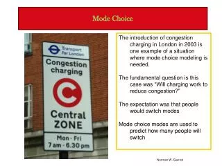
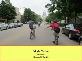
Mode Choice Lecture 10 Norman W. Garrick. Mode Choice. The introduction of congestion charging in London in 2003 is one example of a situation where mode choice modeling is needed. The fundamental question is this case was “ Will charging work to reduce congestion? ”

E N D
Mode Choice Lecture 10 Norman W. Garrick
Mode Choice The introduction of congestion charging in London in 2003 is one example of a situation where mode choice modeling is needed. The fundamental question is this case was “Will charging work to reduce congestion?” The expectation was that people would switch modes Mode choice modes are used to predict how many people will switch Norman W. Garrick
Mode Choice: London Congestion Charging 0.75 mile Norman W. Garrick
Mode Choice: London Congestion Charging Source: http://www.flickr.com/photos/astrolondon/224826598/ These are some of London's congestion charging camera's. They monitor all vehicles entering through the London congestion charge boundary zone and automatically issue a bill to owner of the vehicle. There are thousands of these all around the perimeter of the "C" zone. Transport for London Link http://www.tfl.gov.uk/tfl/roadusers/congestioncharge/whereandwhen/ Norman W. Garrick
Mode Choice The introduction of the new AVE service between Madrid and Barcelona is another example of a situation were model choice modeling would be needed. How many people would switch from plane or driving to train? http://www.renfe.es/video.html Norman W. Garrick
Factors affecting Mode Choice Earlier in the semester we talked about some of the factors affecting mode choice. These factors include 1. Type and purpose of trip 2. Car ownership status 3. Cost (mostly out of pocket cost) 4. Door-to-door travel time 5. Convenience/service/comfort 6. Prestige 7. Availability 8. Accessibility of mode 9. Land use characteristics of start and end point Obviously, not all of these factors can be effectively incorporated into a quantitative model of mode choice. We need to be cognizant of those factors that are important in influencing choice but are not fully accounted for in mode choice models. Norman W. Garrick
Mode Split or Modal Choice Models Mode Choice Models are used to try to predict travelers mode choice Contemporary models are based on using UTILITY or DISUTILITY functions These functions are meant to express the level of satisfaction (for utility functions) or dissatisfaction (for disutility functions) with a given mode Once the utility function is calculated for each mode, the probability that a given mode will be chosen can then be calculated Norman W. Garrick
Utility Function A utility function takes the following form uk = ak + a1 X1 + a2 X2 + ….. ar Xr + ε0 Where uk – utility function for mode k ak – modal constant Xr – variables measuring modal attributes such as cost or time of travel ar – coefficient associated with each attribute ε0 – error term Norman W. Garrick
Multinomial Logit Model If utility function, uk, is assumed to be a Weibull Probability Distribution then the Multinomial Logit Model is used to calculate the probability that a traveler will chose a given mode Multinomial Logit Model p(k) = euk / Σ euk Norman W. Garrick ε0 – error term
Example • The mode available between Zone I and J are i) Automobile (A), ii) Bus (B) • Find the market share for each mode given the attribute table (on next page) for the modes. • The utility function is • uk = ak – 0.025 X1 – 0.032 X2 – 0.015 X3– 0.002 X4 • where • x1 – access plus egress time (min) • x2 – waiting time (min) • x3 – line haul time (min) • x4 – out of pocket cost (cents) Norman W. Garrick
Example … continue The attribute table for each mode is given below And aa = -0.10 ab = +0.00 Therefore u(A) = -0.625 u(B) = -1.530 Probability of selecting PC, p(A) = e(-0.625) / [e(-0.625)+e(-1.530)] = 0.71 Norman W. Garrick