Trip Generation and Mode Choice
Trip Generation and Mode Choice. CEE 320 Steve Muench. Outline. Trip Generation Mode Choice Survey. Trip Generation. Purpose Predict how many trips will be made Predict exactly when a trip will be made Approach Aggregate decision-making units Categorized trip types


Trip Generation and Mode Choice
E N D
Presentation Transcript
Trip Generationand Mode Choice CEE 320Steve Muench
Outline • Trip Generation • Mode Choice • Survey
Trip Generation • Purpose • Predict how many trips will be made • Predict exactly when a trip will be made • Approach • Aggregate decision-making units • Categorized trip types • Aggregate trip times (e.g., AM, PM, rush hour) • Generate Model
Motivations for Making Trips • Lifestyle • Residential choice • Work choice • Recreational choice • Kids, marriage • Money • Life stage • Technology
Reporting of Trips - Issues • Under-reporting trivial trips • Trip chaining • Other reasons (passenger in a car for example)
Trip Generation Models • Linear (simple) • Poisson (a bit better)
Poisson Distribution • Count distribution • Uses discrete values • Different than a continuous distribution
Poisson Ideas • Probability of exactly 4 trips being generated • P(n=4) • Probability of less than 4 trips generated • P(n<4) = P(0) + P(1) + P(2) + P(3) • Probability of 4 or more trips generated • P(n≥4) = 1 – P(n<4) = 1 – (P(0) + P(1) + P(2) + P(3)) • Amount of time between successive trips
Poisson Distribution Example Trip generation from my house is assumed Poisson distributed with an average trip generation per day of 2.8 trips. What is the probability of the following: • Exactly 2 trips in a day? • Less than 2 trips in a day? • More than 2 trips in a day?
Example Calculations Exactly 2: Less than 2: More than 2:
Example Recreational or pleasure trips measured by λi (Poisson model):
Example • Probability of exactly “n” trips using the Poisson model: • Cumulative probability • Probability of one trip or less: P(0) + P(1) = 0.52 • Probability of at least two trips: 1 – (P(0) + P(1)) = 0.48 • Confidence level • We are 52% confident that no more than one recreational or pleasure trip will be made by the average individual in a day
Mode Choice • Purpose • Predict the mode of travel for each trip • Approach • Categorized modes (SOV, HOV, bus, bike, etc.) • Generate Model
Dilemma Qualitative Dependent Variable Explanatory Variables
Dilemma = observation 1 Walk to School (yes/no variable) 1 = no, 0 = yes 0 0 10 Home to School Distance (miles)
A Mode Choice Model • Logit Model • Final form Specifiable part Unspecifiable part s = all available alternatives m = alternative being considered n = traveler characteristic k = traveler
Discrete Choice Example Regarding the TV sitcom Gilligan’s Island, whom do you prefer?
Ginger Model UGinger = 0.0699728 – 0.82331(carg) + 0.90671(mang) + 0.64341(pierceg) – 1.08095(genxg)
Mary Anne Model UMary Anne = 1.83275 – 0.11039(privatem) – 0.0483453(agem) – 0.85400(sinm) – 0.16781(housem) + 0.67812(seanm) + 0.64508(collegem) – 0.71374(llm) + 0.65457(boomm)
No Preference Model Uno preference = – 9.02430x10⁻⁶(incn) – 0.53362(gunsn) + 1.13655(nojames) + 0.66619(cafn) + 0.96145(ohairn)
Results Average probabilities of selection for each choice are shown in yellow. These average percentages were converted to a hypothetical number of respondents out of a total of 207.
Primary References • Mannering, F.L.; Kilareski, W.P. and Washburn, S.S. (2005). Principles of Highway Engineering and Traffic Analysis, Third Edition. Chapter 8 • Transportation Research Board. (2000). Highway Capacity Manual 2000. National Research Council, Washington, D.C.