Interpreting Large Scale Structure
This paper delves into advancements in Large Scale Structure (LSS) studies, emphasizing the dynamics between galaxies and dark matter across cosmic scales. It explores significant surveys including the 2dFGRS, SDSS, and the impact of weak lensing on galaxy-matter correlations. The investigations tackle fundamental questions on the universe's matter-energy content, the nature of dark energy, and the physical processes influencing galaxy formation. By integrating various cosmological data sources, this work aims to refine models that connect galaxies and dark matter through improved measurements and theoretical frameworks.

Interpreting Large Scale Structure
E N D
Presentation Transcript
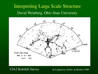
Interpreting Large Scale Structure David Weinberg, Ohio State University CfA2 Redshift Survey de Lapparent, Geller, & Huchra 1986
Las Campanas Redshift Survey Shectman et al. 1996
Sloan Digital Sky Survey Image courtesy of M. Tegmark
Sloan Digital Sky Survey Volume-limited sample Mr < -20 Berlind et al. 2005
Important Developments in LSS Large surveys: dynamic range, precision, detail. Precise measurements for well defined classes of galaxies. Combination of LSS constraints with CMB, other cosmological data. 3. Improved modeling of relation between galaxies and dark matter. 4. Weak lensing: galaxy-matter cross-correlation, matter auto-correlation. 5. Galaxy clustering at high redshift. 6. Matter clustering at high redshift from Ly forest.
Fundamental Questions 1. What are the matter and energy contents of the universe? What is the dark energy accelerating cosmic expansion? 2. What physics produced primordial density fluctuations? 3. Why do galaxies exist? What physical processes determine their masses, sizes, luminosities, colors, and morphologies?
Key issue: relation between galaxies and mass Large scales: gal = f(f ’(0) b Pgal(k) = b2 P(k). Use P(k) shape for cosmology. Also: Redshift space disortions: constrain m0.6 / b Bispectrum: constrain b
SDSS Galaxy Power Spectrum (DR2) • Tegmark et al. 2004: • Redshift real space P(k) recovery • Decorrelated power estimates • Model with linear bias m h = 0.213 +/- 0.023 for b / m = 0.17, ns=1, h=0.72 Tegmark et al. 2004
SDSS Galaxy Power Spectrum (DR2) Tegmark et al. 2004
2dFGRS Galaxy Power Spectrum (final) • Cole et al. 2005: • Angle-averaged redshift space P(k) • Compare to models convolved with survey window function • Model scale-dependent bias as b(k)=(1+Qk2)(1+Ak)-1 • Theory used to motivate form, give priors on parameter values. Cole et al. 2005
2dFGRS Galaxy Power Spectrum (final) m h = 0.168 +/- 0.016 b / m = 0.185 +/- 0.046 For ns=1, h=0.72 Cole et al. 2005
2dFGRS Galaxy Power Spectrum + WMAP CMB m = 0.237 +/- 0.020 b = 0.041 +/- 0.002 h = 0.74 +/- 0.02 ns = 0.954 +/- 0.023 Sanchez et al. 2005
Consistency? Cole et al. 2005
Consistency? Best-fit parameters linear P(k) Cole et al. 2005
Acoustic Peaks in the SDSS Luminous Red Galaxy Sample Eisenstein et al. 2005
Acoustic Peaks in the SDSS Luminous Red Galaxy Sample Eisenstein et al. 2005
SDSS LRGs over 4 orders of magnitude in r Masjedi et al. 2005
SDSS LRGs with Photometric Redshifts Solid: m=0.3, h=0.7 Dotted: Sanchez et al. parameters Padmanabhan et al. 2005
Galaxies vs. Mass: Beyond Linear Bias Dark matter clustering is straightforward to predict for specified initial conditions and cosmological parameters. But where are the galaxies?
Galaxies vs. Mass: Beyond Linear Bias One solution: add gas dynamics and star formation to simulations. Weinberg et al. 2004
Galaxies vs. Mass: Beyond Linear Bias One solution: add gas dynamics and star formation to simulations. Another solution: add semi-analytic galaxy formation to N-body simulations. Weinberg et al. 2004
Galaxies vs. Mass: Beyond Linear Bias One solution: add gas dynamics and star formation to simulations. Another solution: add semi-analytic galaxy formation to N-body simulations. Physical. Challenging. Uncertain. Weinberg et al. 2004
alo Occupation Distribution (HOD): Characterize galaxy-dm relation at halo level, by P(N|M). HOD describes bias for all statistics, on all scales. Predict from theory. Derive empirically from clustering data. Weinberg 2002
P(N|M), SPH simulation Mean occupation, SPH & SA Berlind et al. 2003
P(N|M), SPH simulation Central-satellite separtion Berlind et al. 2003 Zheng et al. 2005
Theory predicts that, to a good approximation, a halo’s galaxy content depends (statistically) on its mass, but not on its larger scale environment. Berlind et al. 2003
Predicted HOD depends strongly on galaxy’s stellar population age. Environment dependence of halo mass function leads to type-dependence of galaxy clustering (e.g., morphology-density relation). Berlind et al. 2003
Galaxy 2-point correlation function gg(r) = excess probability of finding a galaxy a distance r from another galaxy 1-halo term: galaxy pairs in the same halo 2-halo term: galaxy pairs in separate halos
Projected correlation function of SDSS galaxies: Not quite a power law! Zehavi et al. (2004a)
2-halo term 1-halo term Dark matter correlation function Divided by the best-fit power law Deviation naturally explained by HOD model. Zehavi et al. (2004)
Power-law deviations more pronounced at high redshift. 0-parameter “fit” to Ouchi et al.’s (2005) Subaru data at z ~ 4. Conroy, Wechsler, & Kravtsov 2005
For known cosmology, use observed clustering to derive HOD, learn about galaxy formation.
Luminosity dependence of correlation function and HOD Zehavi et al. (2005)
Minimum halo mass vs. luminosity threshold Observation Theory Zheng et al. (2004) Zehavi et al. (2004b)
Color dependence of correlation function Zehavi et al. (2005)
Qualitative agreement with theoretical predictions Berlind et al. (2003), Zheng et al. (2005) Zehavi et al. (2005)
Constrain HOD and cosmological parameters simultaneously. Use intermediate and small scale clustering to break degeneracy between cosmology and galaxy bias.
m = 0.3, 8 = 0.95 m = 0.1, 8 = 0.95 Tinker et al. (2005) m = 0.3, 8 = 0.80
Cluster mass-to-light ratios Given P(k) shape, 8 , choose HOD parameters to match projected correlation function. Predict cluster M/L ratios. These are above or below universal value depending on 8/ 8g . 8=0.95 8=0.8 8=0.6 Tinker et al. (2005)
Cluster mass-to-light ratios Matching CNOC M/L’s implies (8/0.9)(m/0.3)0.6 = 0.71 0.05. Similar results by van den Bosch et al., modeling 2dFGRS. 8=0.95 8=0.8 8=0.6 Tinker et al. (2005)
Breaking degeneracy between cosmology and galaxy bias: Response of clustering observables to cosmological and HOD parameters. Zheng & Weinberg (2005) cosmology P(N|M) internal
Forecast of joint constraints on m and 8, for fixed P(k) shape. Eight clustering statistics, 30 “observables”, each with 10% fractional error. Zheng & Weinberg (2005)
Constrain HOD by fitting wp(rp). Use derived HOD to calculate scale-dependent bias for large scale P(k). Can also use HOD to improve modeling of large scale redshift-space distortions. Yoo, Weinberg, Tinker, in prep.
Conclusions • We’ve come a long way since 1986
Conclusions • We’ve come a long way since 1986 • Large scale P(k) + CMB + etc. • Convergence of results? What parameter values? • HOD framework: • Connects clustering to galaxy formation physics. • Explains power-law deviations in (r) . • Qualitative agreement with theory on luminosity, color dependence. • Use small/intermediate scale clustering to pin down galaxy bias for given cosmology. • Dynamical evidence suggests low 8 and/or m.
Conclusions • We’ve come a long way since 1986 • Large scale P(k) + CMB + etc. • Convergence of results? What parameter values? • HOD framework: • Connects clustering to galaxy formation physics. • Explains power-law deviations in (r) . • Qualitative agreement with theory on luminosity, color dependence. • Use small/intermediate scale clustering to pin down galaxy bias for given cosmology. • Dynamical evidence suggests low 8 and/or m. • Doing precision cosmology is hard.