Download
1 / 41
410 likes | 541 Vues
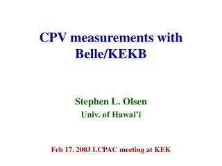
CPV measurements with Belle/KEKB. Stephen L. Olsen Univ. of Hawai’i. Feb 17, 2003 LCPAC meeting at KEK. f 1 : interfere B f CP with B B f CP. ( b ). J/ y. Sanda, Bigi & Carter:. V cb. B 0. K S. . V* 2 sin2 f 1. +. td. J/ y. V*. V tb. td. V cb.

E N D
CPV measurements with Belle/KEKB Stephen L. Olsen Univ. of Hawai’i Feb 17, 2003 LCPAC meeting at KEK
f1 : interfere BfCPwith BBfCP (b) J/y Sanda, Bigi & Carter: Vcb B0 KS V*2 sin2f1 + td J/y V* Vtb td Vcb (akasin2b) B0 B0 B0 KS V* Vtb td td theory errors ~1%
sin2f1 = 0.719±0.074±0.035 B - B B + B more B tags (tags) z more B tags t z/c βγ Now an established & well understood expt’l technique
Agree on value, not name!! Belle & BaBar agree sin2f1 (BaBar) =0.741±0.067±0.033 sin2f1 (Belle) =0.719±0.074±0.035 sin2f1 (World Av.) =0.734±0.055 Agrees with SM theory errors ~1%
What’s next? • sin2f1 shift to precision measurement mode • high statistics • better control of systematics • measure other angles • start with f2 • measure sin2f1 in non-ccs decay modes • sensitive to new physics
f2 (a) from Bp+p- V p+ ub B0 p- + V*2 V2 sin2f2 td ub V* V p- Vtb ub td (akasin2a) B0 B0 p+ Vtb V* td
Must deal with “Penguin Pollution” i.e. additional, non-tree amplitudes with different strong & weak phases * Vtb Vtd p- B0 p+ direct CPV mixing-induced CPV Rq(Dt) 1+q [Appcos(DmDt) + Sppsin(DmDt)] q=+1 B0 tag -1 B0 tag
+0.38 +0.16 -0.27 -0.13 Spp = -1.21 App = +0.94 0.09 (stat.) (syst.) +0.25 -0.31 First results from Belle (Mar 02) “Study of CPV Asymmetries in B0 p+p– Decays” PRL 89, 071801 (2002) • 45 million B-meson pairs (42fb-1) • 162 events in the signal region Results indicate large CP asymmetries, outside of A2+S21 allowed region -5 0 5 Dt (ps)
Outside physical region & some (~2s) disagreement with BaBar
Changes since last March • More data ! [85106B pairs (78 fb-1)] • Analysis improvements: • better track reconstruction algorithm • more sophisticated Dt resolution function • inclusion of additional signal candidates by optimizing event selection • Thorough frequentist statistical analyses • use of Monte Carlo (MC) pseudo-experiments based on control samples
Event and time reconstruction (3) B0 p+p– Selection Flavor tagging Continuum suppression Vertex and Dt Flow • e+e- qq (q=u,d,s,c) continuum background suppression • Event topology • Modified Fox-Wolfram moments • Fisher discriminants • Angular distribution • B flight direction • Combined into a single likelihood ratio • Select 2 regions for each flavor tag class • LR > 0.825 • LRmin < LR 0.825 p+p- (MC) continuum class 1 class 2 class 3 class 4 class 5 class 6 0.825 LRmin
B0 p+p- example p+ p-
B0 p+p–candidates LR > 0.825 LRmin < LR ≤ 0.825 p+p- : 106 Kp : 41 qq : 128 total : 275 p+p- : 57 Kp : 22 qq : 406 total : 485
Event and time reconstruction (4) B0 p+p– Selection Flavor tagging Continuum suppression Vertex and Dt Flow Vertex reconstruction • The same algorithm as that used for sin2f1 meas. • Resolution mostly determined by the tag-side vtx. • B lifetime demonstration with 85 million B pairs B0gD+p-, D*+p-, D*+r-, J/yKS and J/yK*0 B0 lifetime 1.5510.018(stat) ps (PGD02: 1.5420.016 ps) Example vertices Time resolution (rms) 1.43ps
Time-dependent fit Unbinned maximum-likelihood fit (no physical-region constraint) 2 free parameters (App , Spp) in the final fit DE-Mbc dist. B0gD+p-, D*+p-, D*+r-, J/yKS and J/yK*0 (single Gaussian outlier) Lifetime fit The fit program reproduces our sin2f1 results
Reconstruction summary • Established techniques for • event selection • background rejection • flavor tagging • vertexing • time-difference (Dt) fit • In particular, background well under control Common techniques used for branching fractions, Dmd, tB, sin2f1 Now we are able to obtain App and Spp.But let’s go through several crosschecksbefore opening the box.
B0 K+p–control sample Positively-identified kaons (reversed particle-ID requirements w.r.t. pp selection) LR > 0.825 LRmin < LR ≤ 0.825 total Kp yield: 610 events
+0.05 Dmd=0.55 ps-1 0.07 Mixing fit using B0K+p Consistent with the world average (0.4890.008) ps-1 PDG2002 (OFSF)/(OF+SF)
Lifetime measurements world average (PDG2002) (1.542 0.016) ps pp : tB=(1.42 0.14) ps Very different bkgnd fracs Kp : tB=(1.46 0.08) ps BG shape fit background treatment is correct !
CP fits to the BKp sample q=+1 q=-1 SKp = 0.08 0.16 AKp =0.03 0.11 (consistent with counting analysis) No asymmetry
Null asymmetry tests Null asymmetry A = 0.0150.022 S = 0.045 0.033 Null asymmetry
-5 -5 0 0 5 5 p+p- fit results After background subtraction Asymmetry with background subtracted Still see a large CP Violation!
-5 0 5 Fit results App = +0.77 0.27(stat) 0.08(syst) Spp = 1.23 0.41(stat) (syst) +0.08 0.07 After background subtraction Asymmetry with background subtracted data points with LR > 0.825 curves from combined fit result
Likelihoods & errors The probability for such small Spp errors is ~1.2% ln(L) is not parabolic • we use most probable errors from toy-MC
Fit results: App = +0.77 0.27(stat) 0.08(syst) Spp= 1.23 0.41(stat) (syst) How often are we outside the physical region ? +0.08 0.07 Probability that we have a fluctuation equal to or larger than the fit to data (input values at the physical boundary) 16.6% Physical region App2 + Spp2≤ 1 [Note] prob. outside the boundary 60.1% (~independent of statistics)
Prev result App Spp 0.94 -1.21 Cross-checks
(App,Spp) CL regions 3.4s Evidence for CP violation in B0 p+p–
Constraining f2 App | P/T| = 0. 276 0.064 (Gronau-Rosner PRD65, 013004 (2002) Spp
Constraints on f2 allowed regions • Input values for f1 and |P/T| • f1=23.5 (sin2f1=0.73) • |P/T| = 0.3 • f2 constraint w/o isospin analysis ! • both App and Spp large • less restrictive on d • d< 0 favored • no constraint on d at 3s f2 (deg.) d (deg.)
Constraints on f2 (cont’d) ( f1 = 23.5) |P/T| dependence |P/T| = 0.15 |P/T| = 0.45 |P/T| = 0.30 f2 (deg.) d (deg.) • Consistent with theoretical predictions • Larger |P/T| favored
Constraints on f2 78 ≤ f2≤ 152 (for: 0.15|P/T|0.45) f2
(95.5% C.L.) 78 ≤ f2≤ 152 f1 dependence is small
Strategies for f3 Gronau, London, Wyler D0CP K Vub Vcb D0CP 3 2 K Amax ~ 2R ~ 0.2 @ 78 fb –1 47 CP-even evts 50 CP-odd evts A = 0.12 ± 0.13 @500 fb –1: dA/Amax~0.3
Strategies for f3 (cont’d) Atwood, Dunietz, Soni doubly Cabibbo-suppressed Vub Vcb Amax ~ 1; but rate is small Only ~ 15 Dop evts, Cabibbo-suppressed DoK down by ~1/20 80 fb –1: BDop K+p- This strategy is very clean but requires lots & lots of data Mbc
Measure sin2f1 using loop-dominated processes: eff Example: no SM weak phases , ’, K+K- SM: sin2f1 =sin2f1 from BJ/y KS unless there are other, non-SM particles in the loop eff
similar to m(g-2) look for effects of heavy new particles in a well understood SM loop process • well defined technique & target • theory & expt’l errors are well controlled • errors on SM expectationsare small (~5%) • SM terms are highly suppressed • SM loops contain t-quarks & W-bosons • effects of heavy non-SM particles can be large m(g-2): sin2f1eff: lowest-order SM diagrams SM loop particles:t & W SM loop particle: g look for pp1 effects (i.e.~100%) look for ppm effects
These channels are very clean& the techniques are understood Won’t reach experimental limits until ~100x more data
sin2f1eff results: (SM: sin2f1=+0.72± 0.05) 78fb-1 (hep-ex/0212062)PRD(r) B fKS BK+K-KS Bh’KS Spp: -0.73 ± 0.66 +0.52 ± 0.47 +0.76 ± 0.36 2.2σoff OK OK
CPV with Belle (summary) • f1 well established • next: high precision measurements • f21st expt’l limits are established • interesting near future • f3 just beginning • non-SM phases search has begun • 2.2 s discrepancy seen in fKS • BaBar has seen a similar discrepancy in fKS
Conclusion • We’ve accomplished a lot in CPV • There is still a lot more to be done • KEKB & Belle are up to the task