Download
1 / 70
730 likes | 1.61k Vues
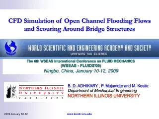
S. Patil, M. Kostic and P. Majumdar Department of Mechanical Engineering NORTHERN ILLINOIS UNIVERSITY. Computational Fluid Dynamics Simulation of Open-Channel Flows Over Bridge-Decks Under Various Flooding Conditions.

E N D
S. Patil, M. Kostic and P. Majumdar Department of Mechanical Engineering NORTHERN ILLINOIS UNIVERSITY Computational Fluid Dynamics Simulationof Open-Channel Flows Over Bridge-DecksUnder Various Flooding Conditions The 6th WSEAS International Conference on FLUID MECHANICS (WSEAS - FLUIDS'09)Ningbo, China, January 10-12, 2009 www.kostic.niu.edu
Motivation: • Bridges are crucial constituents of the nation’s transportation systems • Bridge construction is critical issue as it involves great amount of money and risk • Bridge structures under various flood conditions are studied for bridge stability analysis • Such analyses are carried out by scaled experiments to calculate drag and lift coefficients on the bridge • Scaled experiments are limited to few design variations and flooded conditions due to high cost and time associated with them • Advanced commercial Computational Fluid Dynamics (CFD) software and parallel computers can be used to overcome such limitations www.kostic.niu.edu
CFD is the branch of fluid mechanics which uses numerical methods to solve fluid flow problems • In spite of having simplified equations and high speed computers, CFD can achieve only approximate solutions • CFD is a versatile tool having flexibility is design with an ability to impose and simulate real time phenomena • CFD simulations if properly integrated can complement real time scaled experiments • Available CFD features and powerful parallel computers allow to study wide range of design variations and flooding conditions with different flow characteristics and different flow rates • CFD simulation is a tool for through analysis by providing better insight of what is virtually happening inside the particular design www.kostic.niu.edu
Literature Review: • Ramamurthy, Qu and Vo, conducted simulation of three dimensional free surface flows using VOF method and found good agreement between simulation and experimental results • Maronnier, Picasso and Rappaz, conducted simulation of 3D and 2D free surface flows using VOF method and found close agreement between simulation and experimental results. • Harlow, and Welch, wrote Navier stokes equations in finite difference forms with fine step advancement to simulate transient viscous incompressible flow with free surface. This technique is successfully applicable to wide variety of two and three dimensional applications for free surface • Koshizuka, Tamako and Oka, presented particle method for transient incompressible viscous flow with fluid fragmentation of free surfaces. Simulation of fluid fragmentation for collapse of liquid column against an obstacle was carried. A good agreement was found between numerical simulation and experimental data www.kostic.niu.edu
Objectives: • The objective of the present studyis to validate commercial code STAR-CD for hydraulic research • The experimental data conducted by Turner Fairbank Highway Research Center (TFHRC) at their own laboratories will be simulated using STAR-CD • The base case of Fr = 0.22 and flooding height ratio, h*=1.5 is simulated with appropriate boundary conditions corresponding to experimental testing • The open channel turbulent flow will be simulated using two different methods • First by transient Volume of Fluid (VOF) methodology and other as a steady state closed channel flow with top surface as slip wall • Drag and lift coefficients on the bridge is calculated using six linear eddy viscosity turbulence model and simulation outcome will be compared with experimental results www.kostic.niu.edu
The suitable turbulence model will be identified which predicts close to drag and lift coefficients • The parametric study will be performed for time step, mesh density and convergence criteria to identify optimum computational parameters • The suitable turbulence model will be used to simulate 13 different flooding height ratio from h*=0.3 to 3 for Fr =0.22 www.kostic.niu.edu
ΔWSimulation=0.00254 S=0.058 m LBridge =0.34 m LFlow = 0.26 m Flow Direction Experimental Data: • Experiments are conducted for open channel turbulent flow over six girder bridge deck for different flooding height ratios (h*) and with various flow conditions (Fr) Schematic of experimental six girder bridge deck model www.kostic.niu.edu
LFlow Y X Theory Dimensions of experimental six girder bridge deck model Froude Number Flooding Ratio Nomenclature for bridge dimensions and flooding ratios www.kostic.niu.edu
Experimental data consists of drag and lift coefficients as the function of Froude number, Fr and dimensionless flooding height ratio h* • Experimental data consists of five different sets of experiments for Froude numbers from Fr =0.12 to 0.40 and upstream average velocity 0.20 m/s to 0.65 m/s • The experiments for the Froude number, Fr=0.22 are repeated four times with an average velocity of 0.35 m/s for h*=0.3 to 3 • The lift coefficient is calculated by excluding buoyancy forces in Y (vertical) direction www.kostic.niu.edu
Governing Equations for fluid flow: • Mass conservation equation • Momentum conservation equation • Energy conservation equation www.kostic.niu.edu
y b Dimensionless parameters for open channel flow: • Reynolds Number For 2D open channel flow , www.kostic.niu.edu
Froude Number: • Froude number is dimensionless number which governs character of open channel flow The flow is classified on Froude number Subcritical or tranquil flow Critical Flow Supercritical or rapid flow Open channel flow is dominated by inertial forces for rapid flow and by gravity forces for tranquil flow www.kostic.niu.edu
Froude number is also given by Where Wave speed (m/s) = Flow depth (m) www.kostic.niu.edu
Force Coefficients: • The component of resultant pressure and shear forces in direction of flow is called drag force and component that acts normal to flow direction is called lift force • Drag force coefficient is • Lift force coefficient is • In the experimental testing, the drag reference area is the frontal area normal to the flow direction. The lift reference area is the bridge area perpendicular to Y direction. www.kostic.niu.edu
Drag and lift reference areas for experimental data: For drag, if ,then drag area is if ,then drag area is For lift, for all ,lift area is www.kostic.niu.edu
Turbulent Flow: • Turbulent flow is complex phenomena dominated by rapid and random fluctuations • Turbulent flow is highly unsteady and all the formulae for the turbulent flow are based on experiments or empirical and semi –empirical correlations • Turbulent Intensity • Turbulence mixing length (m) • Turbulent kinetic energy (m2/s2) www.kostic.niu.edu
Turbulence dissipation rate (m2/s3) • Specific dissipation rate (1/s) www.kostic.niu.edu
Turbulence Models: • Six eddy viscosity turbulence models are studied from STAR-CD turbulence options • Two major groups of turbulence models k-ε and k-ωare studied • The k- ε turbulence model The k-ω turbulence models a. Standard High Reynoldsa. Standard High Reynolds b. Renormalization Group b. Standard Low Reynolds c. SST High Reynolds d. SST Low Reynolds www.kostic.niu.edu
The k-ε High Reynolds turbulence model: • Most widely used turbulent transport model • First two equation model to be used in CFD • This model uses transport equations for k and ε in conjunction with the law-of-the wall representation of the boundary layer The k-ε RNG turbulence model: • This turbulence model is obtained after modifying k-ε standard turbulence model using normalization group method to renormalize Navier Stokes equations • This model takes into account effects of different scales of motions on turbulent diffusion www.kostic.niu.edu
k-ω turbulence model: • The k-ω turbulence models are obtained as an alternative to the k-ε model which have some difficulty for near wall treatment • The k-ω turbulence models Standard k-ω model Shear stress transport (SST) model High Reynolds Low Reynolds High Reynolds Low Reynolds www.kostic.niu.edu
SST k-ω turbulence model: • SST turbulence model is obtained after combining best features of k-ε and k-ω turbulence model • SST turbulence model is the result of blending of k-ω model near the wall and k-ε model near the wall www.kostic.niu.edu
Computational Model: • STAR-CD (Simulation of Turbulent flow in Arbitrary Regions Computational Dynamics) is CFD analysis software • STAR-CD is finite volume code which solves governing equations for steady state or transient problem • The first method used in STAR-CD to simulate open channel turbulent flow is free surface method which makes use of Volume of Fluid (VOF) methodology • VOF methodology simulates air and water domain • VOF methodology uses volume of fraction variable to capture air-water interface www.kostic.niu.edu
VOF technique: • VOF technique is a transient scheme which captures free surface. • VOF deals with light and heavy fluids • VOF is the ratio of volume of heavy fluid to the total control volume • Volume of fraction is given by • Transport equation for volume of fraction • Volume fraction of the remaining component is given by www.kostic.niu.edu
The properties at the free surface vary according to volume fraction of each component www.kostic.niu.edu
0.30 0.08 0.06 0 Y -0.15 X -1.50 1.78 03 0.26 Z Free Surface method: • Dimensions for computational model h*=1.5 generated in STAR-CD (Dimensions not to scale and in SI units) www.kostic.niu.edu
Y X Y Computational Mesh: Full computational domain with non uniform mesh and 2 cells thick in Z direction for =1.5 www.kostic.niu.edu
Bottom Wall (No Slip) Outlet Symmetry Plane Top wall (slip) Air Inlet Water Inlet Y Y X Z Boundary Conditions: www.kostic.niu.edu
Computational parameters for VOF methodology: www.kostic.niu.edu
0.08 0.06 0 Y -0.15 X Z -1.5 03 1.78 0.26 Water slip top wall method: • Dimensions for computational model h*=1.5 for water slip –top-wall method (Dimensions not to scale and in SI units) www.kostic.niu.edu
Symmetry Plane Top wall (slip) Water Inlet Bottom wall (No slip) Outlet (Standard) Y Y X X Boundary conditions: Computational domain with boundary surfaces and boundary conditions for water slip-top-wall method www.kostic.niu.edu
Computational parameters for water slip-top-wall method: Inlet velocity, Turbulent kinetic energy, Turbulent Dissipation Rate, www.kostic.niu.edu
STAR-CD simulation Validation with basics of fluid mechanics : Fully developed velocity profile for laminar pipe flow after STAR-CD simulation www.kostic.niu.edu
Fully developed velocity profile for the turbulent pipe flow after STAR-CD simulation www.kostic.niu.edu
Comparison between theoretical and simulated friction factor : www.kostic.niu.edu
Calculation of entrance length: Continued on next page www.kostic.niu.edu
Verification of power law velocity profile: www.kostic.niu.edu
Y X 1.016 0.504 0 0.254 0.127 0.097 0 Comparison between Fluent and STAR-CD for same geometry: www.kostic.niu.edu
Comparison for velocity contours between STAR-CD and Fluent www.kostic.niu.edu
Comparison for velocity vectors between STAR-CD and Fluent www.kostic.niu.edu
Comparison for X velocities between Fluent and STAR-CD www.kostic.niu.edu
Pressure difference (Pa) Force Coefficients Force Coefficients Fluent STAR-CD (Reference Data) Absolute Difference Percentage Difference CD 1.89 2.00 0.11 5.5 % CL -6.77 -7.05 0.28 3.97 % www.kostic.niu.edu
VOF simulation of experimental data: Effect of time steps on drag coefficients www.kostic.niu.edu
Effect of time steps on lift coefficients: www.kostic.niu.edu
Effect of decreased downstream length on force coefficients www.kostic.niu.edu
Effect of decrease in under bridge water depth www.kostic.niu.edu
Effect of top boundary condition at top as slip wall and symmetry www.kostic.niu.edu
Free surface, Free Surface Development: Nomenclature for VOF contour plot Volume fraction for water www.kostic.niu.edu