Download
1 / 33
330 likes | 469 Vues
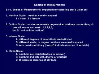
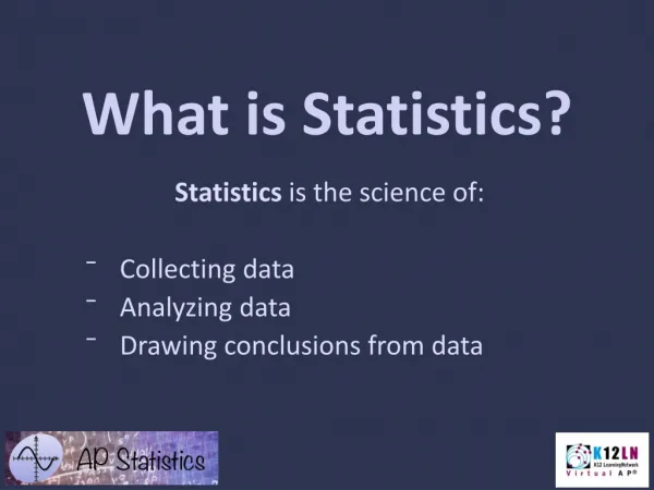
Intro to Statistics Various Variables Scales of Measurement Taking Measurements Frequency Distributions Descriptive Statistics. VI. Descriptive Statistics A. Measures of CENTRAL TENDENCY 1. Mode - the most frequent category or value. VI. Descriptive Statistics

E N D
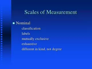
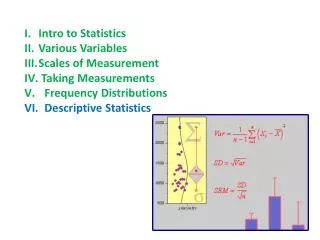
Intro to Statistics • Various Variables • Scales of Measurement • Taking Measurements • Frequency Distributions • Descriptive Statistics
VI. Descriptive Statistics A. Measures of CENTRAL TENDENCY 1. Mode - the most frequent category or value
VI. Descriptive Statistics A. Measures of CENTRAL TENDENCY 1. Mode 2. Median - the middle value in ordered, ranked data - represented by q for population - represented by M for a sample
VI. Descriptive Statistics A. Measures of CENTRAL TENDENCY 1. Mode 2. Median 3. Mean - arithmetic average; most common measure of central tendency for interval/ratio scale.
VI. Descriptive Statistics A. Measures of CENTRAL TENDENCY 1. Mode 2. Median 3. Mean 4. Comparisons - the mean is the most ‘information rich’, as it is affected by every value in the population/sample. - but because of this, it is more affected by extreme values.
Examples: Consider a sample were the mode is ‘10’ (or ‘red’) because there are 15 cases of this value (or attribute). This descriptor of central tendency doesn’t change if there are 5 ‘9’s’, 8 ‘9’s’, 6 ‘1020’s’, or whatever; as long as no value has a greater frequency. 15 Doesn’t matter; as long as frequencies are less than 15. Doesn’t matter; as long as frequencies are less than 15. 10 RED
Examples: Now, consider the median. We just need to know how many values are above and below ours; the magnitude of those values, and their individual frequencies is unimportant. 15 N values below N values above 10
Examples: Now, consider the mean. The value of each case is included in the computation, so the mean is affected by each value. Changes in the magnitude and frequency of values may change the mean.
Ranked Salaries in 1000’s: • 15 • 17 • 21 • 24 • 27 • 31 • 225 Mode = 21, 27 (bimodal) Median = 24 Mean = 45.33
VI. Descriptive Statistics A. Measures of CENTRAL TENDENCY 1. Mode 2. Median 3. Mean 4. Comparisons 5. Weighted mean – when different items have different degrees of importance (weight).
VI. Descriptive Statistics A. Measures of CENTRAL TENDENCY 1. Mode 2. Median 3. Mean 4. Comparisons 5. Weighted mean – when different items have different degrees of importance (weight). Grade A 4.0 B 3.0 C 2.0 mean = 3.0
VI. Descriptive Statistics A. Measures of CENTRAL TENDENCY 1. Mode 2. Median 3. Mean 4. Comparisons 5. Weighted mean – when different items have different degrees of importance (weight). Grade Credits grade pts A 4.0 2.0 (MayX) 8.0 B 3.0 2.0 (MayX) 6.0 C 2.0 4.0 8.0 Sum = 8.0 22.0 GPA = 22/8 = 2.75
VI. Descriptive Statistics A. Measures of CENTRAL TENDENCY B. Location in a SAMPLE/POPULATION - median – the midpoint in a distribution also the “50th percentile” ½ of the values above and below
VI. Descriptive Statistics A. Measures of CENTRAL TENDENCY B. Location in a SAMPLE/POPULATION - median – the midpoint in a distribution also the “50th percentile” ½ of the values above and below - 1st quartile = 25th percentile: 25% below. - 2nd quartile = 50th percentile - 3rd quartile = 75th percentile - 90th percentile = 90% below.
VI. Descriptive Statistics A. Measures of CENTRAL TENDENCY B. Location in a SAMPLE/POPULATION C. Measures of DISPERSION
VI. Descriptive Statistics A. Measures of CENTRAL TENDENCY B. Location in a SAMPLE/POPULATION C. Measures of DISPERSION 1. Range: affected by only two values, and the most EXTREME values. - statistically – may be of little use - biologically – may be important as physiological/ ecological tolerance limits.
VI. Descriptive Statistics A. Measures of CENTRAL TENDENCY B. Location in a SAMPLE/POPULATION C. Measures of DISPERSION 1. Range: affected by only two values, and the most EXTREME values. 2. Interquartile Range: from 1st to 3rd quartile.
3. Standard Deviation (s, s): The average distance between data points and the mean. xi - x 1 – 3 = -2 4 2 – 3 = -1 1 2 – 2 = -1 1 3 – 3 = 0 0 3 – 3 = 0 0 4 – 3 = 1 1 4 – 3 = 1 1 5 – 3 = 2 4 DATA: 1, 2, 2, 3, 3, 4, 4, 5 MEAN: 24/8 = 3 S = (0) S = (xi – x)2 = 12 THIS IS ALSO CALLED THE “SUM OF SQUARES”
3. Standard Deviation (s, s): The average distance between data points and the mean. xi - x Variance = S2 = (ss)/n-1 1 – 3 = -2 4 2 – 3 = -1 1 2 – 2 = -1 1 3 – 3 = 0 0 3 – 3 = 0 0 4 – 3 = 1 1 4 – 3 = 1 1 5 – 3 = 2 4 DATA: 1, 2, 2, 3, 3, 4, 4, 5 MEAN: 24/8 = 3 S = (0) ss = (xi – x)2 = 12 THIS IS ALSO CALLED THE “SUM OF SQUARES”
An easier formula to calculate “sum of squares”: SS = S(x2) – (Sx)2 n
3. Standard Deviation (s, s): The average distance between data points and the mean. - often want a measure of dispersion in the same units as the mean. - but variance is in squared units – so now we take the square-root of the variance to get the standard deviation. sd = s = s2
3. Coefficient of Variation: If you want to compare the dispersion of two distributions measured on different scales (mice and elephants), you can standardize the sd against the mean. This is the coefficient of variation: s x x100 = C.V.
WRITING PAPERS • General Comments • Structure and Scope of a Review Paper • Structure of a Primary Research Paper • A. Abstract • B. Introduction • C. Methods
C. Methods - What you did and why, in enough detail so it can be replicated - Written in prose – paragraphs - logical flow… maybe temporal, maybe not. Maybe presented in association with specific questions - Past tense… active / passive voice
C. Methods - Include variables (independent variables, controlled variables, uncontrolled variables, maybe not explicitly categorized) - Include all dependent variables and how they were measured. - Include how each dependent variable was analyzed… specific statistical tests and contrasts - Include apparati only if unique or very specific
C. Methods • - Complete taxonomic information • - Important characteristics about • subjects: age, weight, sex, etc. • - Describe tools and supplies • - Cite previous methodology where • appropriate • - Include study site if a field project
WRITING PAPERS • General Comments • Structure and Scope of a Review Paper • Structure of a Primary Research Paper • A. Abstract • B. Introduction • C. Methods • D. Results
D. Results Don’t say: “Figure 1 shows that…” “The data show that…” “The chi-squared tests shows that…”
D. Results Don’t say: “Figure 1 shows that… mass is inversely correlated with density” “The data show that… abundance declines with density” “The chi-squared tests shows that… the gene exhibits complete dominance.”
D. Results Don’t say: “Mass is inversely correlated with density (Fig. 1).” “Abundance declines with density (Fig. 2).” “The gene exhibits complete dominance (Chi-squared test, X2 = 35.63, p = 0.001).”