Chapter 3 Aggregate Planning
Chapter 3 Aggregate Planning. Introduction to Aggregate Planning. Goal: To plan gross work force levels and set firm-wide production plans.

Chapter 3 Aggregate Planning
E N D
Presentation Transcript
Introduction to Aggregate Planning • Goal: To plan gross work force levels and set firm-wide production plans. Concept is predicated on the idea of an “aggregate unit” of production. May be actual units, or may be measured in weight (tons of steel), volume (gallons of gasoline), time (worker-hours), or dollars of sales. Can even be a fictitious quantity. (Refer to example in text and in slide below.)
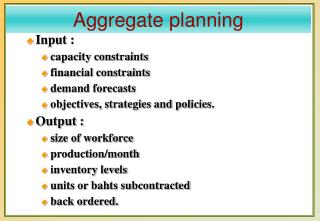
Overview of the Problem Suppose that D1, D2, . . . , DT are the forecasts of demand for aggregate units over the planning horizon (T periods.) The problem is to determine both work force levels (Wt) and production levels (Pt ) to minimize total costs over the T period planning horizon.
Important Issues • Smoothing. Refers to the costs and disruptions that result from making changes from one period to the next. • Bottleneck Planning. Problem of meeting peak demand because of capacity restrictions. • Planning Horizon. Assumed given (T), but what is “right” value? Rolling horizons and end of horizon effect are both important issues. • Treatment of Demand. Assume demand is known. Ignores uncertainty to focus on the predictable/systematic variations in demand, such as seasonality.
Relevant Costs • Smoothing Costs • changing size of the work force • changing number of units produced • Holding Costs • primary component: opportunity cost of investment • Shortage Costs • Cost of demand exceeding stock on hand. Why should shortages be an issue if demand is known? • Other Costs: payroll, overtime, subcontracting.
$ Cost Slope = Ci Slope = CP Back-orders Positive inventory Inventory Holding and Back-Order Costs
Aggregate Units The method is based on notion of aggregate units. They may be • Actual units of production • Weight (tons of steel) • Volume (gallons of gasoline) • Dollars (Value of sales) • Fictitious aggregate units
Example of fictitious aggregate units.(Example 3.1) One plant produced 6 models of washing machines: Model # hrs. Price % sales A 5532 4.2 285 32 K 4242 4.9 345 21 L 9898 5.1 395 17 L 3800 5.2 425 14 M 2624 5.4 525 10 M 3880 5.8 725 06 Question: How do we define an aggregate unit here?
Example continued • Notice: Price is not necessarily proportional to worker hours (i.e., cost): why? • One method for defining an aggregate unit: requires: .32(4.2) + .21(4.9) + . . . + .06(5.8) = 4.8644 worker hours. Forecasts for demand for aggregate units can be obtained by taking a weighted average (using the same weights) of individual item forecasts.
Prototype Aggregate Planning Example(this example is not in the text) The washing machine plant is interested in determining work force and production levels for the next 8 months. Forecasted demands for Jan-Aug. are: 420, 280, 460, 190, 310, 145, 110, 125. Starting inventory at the end of December is 200 and the firm would like to have 100 units on hand at the end of August. Find monthly production levels.
Step 1: Determine “net” demand.(subtract starting inv. from per. 1 forecast and add ending inv. to per. 8 forecast.) Month Net Predicted Cum. Net Days Demand Demand 1(Jan) 220 220 22 2(Feb) 280 500 16 3(Mar) 460 960 23 4(Apr) 190 1150 20 5(May) 310 1460 21 6(June) 145 1605 17 7(July) 110 1715 18 8(Aug) 225 1940 10
Step 2. Graph Cumulative Net Demand to Find Plans Graphically
Constant Work Force Plan Suppose that we are interested in determining a production plan that doesn’t change the size of the workforce over the planning horizon. How would we do that? One method: In previous picture, draw a straight line from origin to 1940 units in month 8: The slope of the line is the number of units to produce each month.
Monthly Production = 1940/8 = 242.2 or rounded to 243/month. But: there are stockouts.
How can we have a constant work force plan with no stockouts? Answer: using the graph, find the straight line that goes through the origin and lies completely above the cumulative net demand curve:
From the previous graph, we see that cum. net demand curve is crossed at period 3, so that monthly production is 960/3 = 320. Ending inventory each month is found from: Month Cum. Net. Dem. Cum. Prod. Invent. 1(Jan) 220 320 100 2(Feb) 500 640 140 3(Mar) 960 960 0 4(Apr.) 1150 1280 130 5(May) 1460 1600 140 6(June) 1605 1920 315 7(July) 1715 2240 525 8(Aug) 1940 2560 620
But - may not be realistic for several reasons: • It may not be possible to achieve the production level of 320 unit/month with an integer number of workers • Since all months do not have the same number of workdays, a constant production level may not translate to the same number of workers each month.
To overcome these shortcomings: • Assume number of workdays per month is given • K factor given (or computed) where K = # of aggregate units produced by one worker in one day
Finding K • Suppose that we are told that over a period of 40 days, the plant had 38 workers who produced 520 units. It follows that: • K= 520/(38*40) = 0.3421 = average number of units produced by one worker in one day.
Computing Constant Work Force Assume we are given the following # of working days per month: 22, 16, 23, 20, 21, 17, 18, 10. March is still critical month. Cum. net demand thru March = 960. Cum # of working days = 22+16+23 = 61. Find 960/61 = 15.7377 units/day implies 15.7377/.3421 = 46 workers required.
Constant Work Force Production Plan Mo # wk days Prod. Cum Cum Net End Inv Level Prod Dem Jan 22 346 346 220 126 Feb 16 252 598 500 98 Mar 23 362 960 960 0 Apr 20 315 1275 1150 125 May 21 330 1605 1460 145 Jun 22 346 1951 1605 346 Jul 21 330 2281 1715 566 Aug 22 346 2627 1940 687
Addition of Costs • Holding Cost (per unit per month): $8.50 • Hiring Cost per worker: $800 • Firing Cost per worker: $1,250 • Payroll Cost: $75/worker/day • Shortage Cost: $50 unit short/month
Cost Evaluation of Constant Work Force Plan • Assume that the work force at end of Dec was 40. • Cost to hire 6 workers: 6*800 = $4800 • Inventory Cost: accumulate ending inventory: (126+98+0+. . .+687) = 2093. Add in 100 units netted out in Aug = 2193. Hence Inv. Cost = 2193*8.5=$18,640.50 • Payroll cost: ($75/worker/day)(46 workers )(167days) = $576,150 • Cost of plan: $576,150 + $18,640.50 + $4800 = $599,590.50 ~ $600K
Cost Reduction in Constant Work Force Plan In the original cum net demand curve, consider making reductions in the work force one or more times over the planning horizon to decrease inventory investment.
Cost Evaluation of Modified Plan • I will not present all the details here. The modified plan calls for reducing the workforce to 36 at start of April and making another reduction to 22 at start of June. The additional cost of layoffs is $30,000, but holding costs are reduced to only $4,250. The total cost of the modified plan is $467,450.
Zero Inventory Plan (Chase Strategy) • Here the idea is to change the workforce each month in order to reduce ending inventory to nearly zero by matching the workforce with monthly demand as closely as possible. This is accomplished by computing the # units produced by one worker each month (by multiplying K by #days per month) and then taking net demand each month and dividing by this quantity. The resulting ratio is rounded up and possibly adjusted downward.
I got the following for this problem: • Period # hired #fired • 1 10 Cost of this • 2 20 plan: • 3 9 $555,704.50 • 4 31 • 5 15 • 6 24 • 7 4 • 8 15
How to disaggregate? • Have to disaggregate a aggregate plan to a master production schedule (MPS) • MPS will then be used to plan for material requirements of the production and detailed scheduling
Optimal Solutions to Aggregate Planning Problems Via Linear Programming Linear Programming provides a means of solving aggregate planning problems optimally. The LP formulation is fairly complex requiring 8T variables and 3T constraints, where T is the length of the planning horizon. Clearly, this can be a formidable linear program. The LP formulation shows that the modified plan we considered with two months of layoffs is in fact optimal for the prototype problem. Refer to the latter part of Chapter 3 and the Appendix following the chapter for details.