3. Aggregate Planning
3. Aggregate Planning. Aggregate Planning. Aggregate Planning. Provides the quantity and timing of production for intermediate future Usually 3 to 18 months into future Combines (‘aggregates’) production Often expressed in common units : h ours, dollars, equivalents


3. Aggregate Planning
E N D
Presentation Transcript
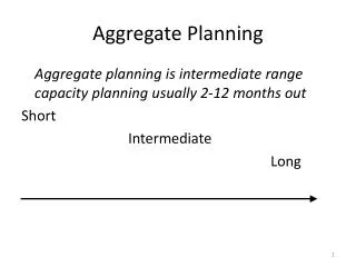
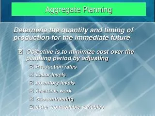
Aggregate Planning • Provides the quantity and timing of production for intermediate future • Usually 3 to 18 months into future • Combines (‘aggregates’) production • Often expressed in common units: hours, dollars, equivalents • Involves capacity and demand variables
Aggregate Planning Goals • Meet demand • Use capacity efficiently • Meet inventory policy • Minimize cost • Labor • Inventory • Plant & equipment • Subcontract
Options to Consider • Changing inventory levels (with backorders) • Varying workforce size by hiring or layoffs • Varying production rates through overtime or idle time • Subcontracting • Using part-time workers • Influencing demand
Aggregate Planning Strategies • Chase Strategy • Matching the production rate to exactly meet the demand by hiring and laying off workers. • Level Strategy • Maintain a stable workforce working at constant output rate; absorb demand variations with inventory, backlogs, or lost sales. • Mixed Strategy • A combination of chase and level strategies to match supply and demand.
Aggregate Planning Methods • Spreadsheet techniques • Popular & easy-to-understand • Trial & error approach • Mathematical approaches • Linear programming models • Simulation
Example • A manufacturer of roofing supplies has monthly forecasts for the 6-month period
Forecast demand 70 – 60 – 50 – 40 – 30 – 0 – Level production using average monthly forecast demand Production rate per working day Jan Feb Mar Apr May June = Month 22 18 21 21 22 20 = Number of working days Continued
Continued • inventory cost: $5/unit, backorder cost: $10/unit • wage: $40/day, hiring cost: $1500, layoff cost: $3000 • production rate: 5 units/day
Linear Programming Models • Workforce planning model • Production planning model
Workforce Planning Model • Decision variables Wt = number of workers available in periodt Ht = number of workers hired in periodt Lt = number of workers laid off in period t Pt = number of units produced in periodt It = number of units in inventory at the end of periodt Bt = number of units backordered at the end of periodt
Continued • Given parameters Dt = demand forecast in periodt nt = number of units made by one worker in periodt CtW = cost of oneworkerin period t CtH, CtL = cost to hire or lay off oneworkerin period t CtP = cost to produce one unit in periodt CtI, CtB = cost to hold or backorder one unit for period t
Continued • Objective function • Constraints • Possible extensions
Mar Apr May Demand 800 1,000 750 Capacity 850 850 850 Beginning inventory 100 Production cost 40 41 45 Inventory cost 2 2 2 Production Planning Model
Model 1 • Pt = number of units produced in periodt It = units in inventory at the end of periodt
Model 2 • Let Xij be the number of items produced in month i and consumed in month j.
Mar Apr May Demand 800 1,000 750 Capacity: Regular 700 700 700 Overtime 50 50 50 Subcontracting 150 150 130 Beginning inventory 100 tires Costs Regular time $40 per tire Overtime $50 per tire Subcontracting $70 per tire Inventory $ 2 per tire per month Another Example
Model 2 • Let Xij, Yij and Zij be the number of items produced in month i and consumed in month j, using regular production, overtime, and subcontracting, respectively.