Download

1 / 30
300 likes | 320 Vues
Learn about the concepts of price elasticity of demand and supply, and how they determine consumer responsiveness to price changes. Explore the Midpoint formula and Total Revenue Test, and understand the determinants of price elasticity.

E N D
A. Price elasticity of demand – responsiveness (sensitivity) of consumers to a price change ($ Δ). • LAW OF DEMAND: • $ = Purchases $ = Purchases Three ideas: • Price elasticity • Cross elasticity – buying response of consumers of one product when the price of another product changes. • Income elasticity – the buying response of consumers when their income changes.
Economists measure the degree of price elasticity or inelasticity of demand with the coefficient Ed, defined as: percentage change in quantity Ed = demanded of product X percentage change in price of product X B. Price-elasticity Coefficient & Formula C. Midpoint formula – simplest solution: Quantity demanded = Qd **USE THIS FORMULA** Δ in QΔ in $ Ed = sum of Q / 2 √ sum of prices / 2 -- % are better than absolute amounts; eliminate the minus sign for clarification. -- Use the Midpoint Formula for the Popcorn simulation.
D. Interpretations of Ed • Elastic demand – % Δ in price results in a larger % Δ in Qd (Ed> 1), Ex: A 2% in $ 4% in Qd Ed = .04 = 2 (demand is elastic) .02 ● Inelastic demand – % Δ in $ results in a smaller % Δ in Qd (Ed< 1), Ex: A 2% in $ 1% in Qd Ed = .01 = .5 (demand is inelastic) .02
Unit elasticity – % Δ in $ and the resulting % Δ in Qd are the same (Ed = 1), Ex: A 2% in $ 2% in Qd Ed = .02 = 1 (unit elasticity) .02 ● Perfectly inelastic (rare) – coefficient is zero due to consumers being unresponsive to a $ Δ.
E. Perfectly inelastic – a $ Δ results in no Δ in demand. F. Perfectly elastic – infinite coefficient (∞). VERTICAL Perfectly Inelastic has relatively little “quantity stretch” HORIZONTAL Perfectly Elastic has considerable “quantity stretch” **Important for Popcorn simulation**
.04 Ed = = 2 .02 .01 Ed = = .5 .02 .02 Ed = = 1 .02 Price Elasticity of Demand • Why Use Percentages? • Elimination of the Minus Sign • Interpretations of Ed Elastic Demand Inelastic Demand Unit Elasticity
P $3 2 1 Q 0 10 20 30 40 The Total Revenue Test • Total Revenue (TR) TR = P x Q Elastic Demand **Use the TR Graph for Popcorn Simulation** 2 X 10 (a) = 20 1 X 40 (b) = 40 Pt ‘b’ is greater a b D1 Ed (Midpoint formula) = Δ in QΔ in $ sum of Q/2 √ sum of $/2
P $4 3 2 1 Q 0 10 20 The Total Revenue Test • Total Revenue (TR) TR = P x Q Inelastic Demand c 4 X 10 (c) = 40 1 X 20 (d) = 20 Pt ‘c’ is greater d Ed (Midpoint formula) = Δ in QΔ in $ sum of Q/2 √ sum of $/2 D2
P $3 2 1 Q 0 10 20 30 The Total Revenue Test • Total Revenue (TR) TR = P x Q Unit-Elastic e f D3
Midpoint Formula – finding the price elasticity coefficient. • Is the demand for tickets elastic or inelastic? • Try using averages of two tickets and two quantities as the reference point. Ed = Δ in quantity√ Δ in $ sum of quantities/2 sum of price/2 Using data from the $5 - $4 price range: Ed = 1 √ 1 = 1 9/2 9/2
G. Total Revenue (TR) – total amount the seller receives from the sale of product in particular time period. **Important for Popcorn simulation** TR = price (P) X quantity (Q) $ & TR = D is elastic. $ & TR is unchanged = D is unit-elastic. $ & TR = D in inelastic -- Firms want to know the effect of price changes on total revenue and thus profits (total revenue minus total costs). -- ‘Total-revenue test’ looks at what happens to TR when product $ Δ. -- Graph: Lowering the tix price from $8 to $5 (elastic range) increased TR. -- Lowering price from $4 to $1 (inelastic range) lowered TR.
Graphical Analysis **Important for Popcorn simulation** • Relationship between price elasticity of demand for movie tickets. • Demand curve D is based on table 20.1. • More price elastic between $5-8 price range of D than between $4-1 range.
$8 7 6 5 4 3 2 1 a b c Price d e f g h 0 0 1 1 2 2 3 3 4 4 5 5 6 6 7 7 8 8 Quantity Demanded $20 18 16 14 12 10 8 6 4 2 Total Revenue (Thousands of Dollars) Quantity Demanded Price Elasticity and the Total-Revenue Curve Elastic Ed > 1 Unit Elastic Ed = 1 Inelastic Ed < 1 Correctly label these two graphs for the Popcorn Simulation! D Elastic Ed > 1 Unit Elastic Ed = 1 TR Inelastic Ed < 1
Determinants of Price Elasticity of Demand • Substitutability ● Luxuries v. Necessities • Proportion of Income ● Time
Applications of Price Elasticity of Demand • Large crop yields • Excise tax • Decriminalize illegal drugs • Minimum wage ($10/CA, $7.25/Fed) Typical examples of excise duties are taxes on gasoline, tobacco and alcohol (sometimes referred to as sin taxes).
H. Price elasticity of Supply – if producers are relatively responsive to $ Δ = supply is elastic; if not = inelastic. % Δ in quantity Es =supply of product X % Δ in $ of product X OR An increase in the $ of a good from $4 to $6 increases the quantity supplied from 10 units to 14 units. The % Δ in $ would be 2/5, or 40%, and the % Δ in quantity would be 4/12, or 33%: .33 Es = .40 = .83 -- The degree of price elasticity of supply depends on how easily (how quickly) producers can shift resources between alternative uses. -- Faster shift = elasticity of supply; Slower response = inelasticity.
Market supply I. Market period Price Elasticity of Supply in Microeconomics -- Market period: period that occurs when the time immediately after a Δ in market price is too short for producers to respond w/ a Δ in quantity supplied. -- Ex: a tomato farmer only has one truck full of tomatoes to sell; line is vertical (perfectly inelastic) due to not having time to respond to change in demand (D1 to D2). -- P0 to Pm determines which buyers get the fixed quantity supplied.
P Q Price Elasticity of Supply Percentage Change in Quantity Supplied of Product X Es = Percentage Change in Price of Product X Unit Elastic Supply Es = 1 Market Period: Not Enough Time to Shift Resources Sm Pm Greatest Price Impact P0 D1 D2 Q0
Price Elasticity of Supply in Microeconomics 1. Short run 2. Long run -- Short run – period of time too short to change plant capacity but long enough to use fixed plant more or less inexpensively (fixed land/farm machinery, but can use more labor/fertilizer) for more output (more elastic). -- Long run – time period long enough for firms to adjust their plant sizes & for new firms to enter (or existing to leave) the industry (still more elastic). -- There is no total-revenue test for elasticity of supply. -- Supply shows a positive (direct relationship) between $ & amount supplied.
P Q Price Elasticity of Supply Percentage Change in Quantity Supplied of Product X Es = Percentage Change in Price of Product X Inelastic Supply Es < 1 Short Run: Resources Not Easily Shifted to Alternative Uses Ss Lower Price Impact Ps P0 D1 D2 Q0 Qs
P Q Price Elasticity of Supply Percentage Change in Quantity Supplied of Product X Es = Percentage Change in Price of Product X Elastic Supply Es > 1 Long Run: Resources Easily Shifted to Alternative Uses Sl Least Price Impact Pl P0 D1 D2 Q0 Ql
J. Cross elasticity of demand – measures how sensitive customers purchases are to 2 products. 1. Substitute goods 2. Complimentary goods 3. Independent goods % Δ in Qd of product X Exy = % Δ in Qd of product Y -- One product is X, the other is Y. -- The cross-price elasticity allows us to quantify/understand substitute and complimentary goods (Ch 3).
K. Income elasticity of demand – measures degree consumers respond to Δ in their incomes by buying more/less of a good. 1. Normal goods 2. Inferior goods % Δ in Qd Ei = % Δ in I -- For most goods, income-elasticity coefficient Ei is positive (more are demanded as income rises); called normal or superior goods. -- Inferior goods have a negative income-elasticity (more $ = lower sales). -- Insights: we do not eat more when our income rises, we eat better! -- When income declines, food purchases stay same but buy fewer electronics.
Cross Elasticity of Demand Percentage Change in Quantity Demanded of Product X Exy = • Substitute Goods – Positive Sign • Complementary Goods- Negative Sign • Independent Goods – Zero or Near-Zero Value Percentage Change in Price of Product Y
Income Elasticity of Demand Percentage Change in Quantity Demanded Ei = • Normal Goods – Positive Sign • Inferior Goods - Negative Sign • Insights into the Economy Percentage Change in Income
Consumer and Producer Surplus Consumer Surplus Use this graph for Popcorn Simulation Consumer Surplus Equilibrium Price = $8 P1 Price (Per Bag) D Q1 Quantity (Bags)
Consumer and Producer Surplus Efficiency Losses (Deadweight Losses) Efficiency Revisited Ch. 22 S Efficiency Losses P1 Price (Per Bag) D Q3 Q2 Q1 Quantity (Bags)