Future Climate Changes: Insights from Models and Scenarios
Chapter 6 explores future climate changes through dynamic modeling and predictive scenarios. It discusses methods for estimating climate responses to various external forcings, including greenhouse gases and aerosols. The chapter highlights the Representative Concentration Pathways (RCP) as well as SRES scenarios, providing insights into projected specific climate outcomes such as surface temperature changes and precipitation distribution. Limitations and uncertainties associated with predictions due to internal variability and model divergence are also interpreted, alongside the importance of mitigation policies in influencing future climate trajectories.

Future Climate Changes: Insights from Models and Scenarios
E N D
Presentation Transcript
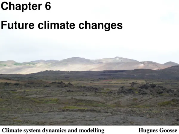
Chapter 6 Future climate changes Climate system dynamics and modelling Hugues Goosse
Outline Methods used to estimate future climate changes. Description of the main results at different timescales. Interpretation and limitations of the predictions. Chapter 6 Page 2
Scenarios • Scenarios for future changes in external forcing have to be selected. • Representative concentration pathways (RCP) scenarios provide a large range of future change in radiative forcing. Chapter 6 Page 3
Scenarios • RCP scenarios provide estimates for future concentration of greenhouse gases, aerosols, land use changes • Global emission (in PgC per year) and (b) atmospheric concentration of CO2 (in ppm) in four RCP scenarios.
Scenarios • SRES scenarios provide estimates for future concentration of greenhouse gases, aerosols, land use changes • Global emissions of sulphur oxide in four RCP scenarios (in TgSO2 per year). Chapter 6 Page 5
Decadal predictions and projections • Projection: goal = estimate the response to the forcing • Boundary condition problem • Predictions: goal = estimate the response to the forcing and the contribution of internal variability (the fraction which is predictable) • Predictions must be initialised using observations. • Mix of initial and boundary condition problem Chapter 6 Page 6
Decadal predictions and projections • Schematic representation of the difference between projections and predictions using one model and one scenario. Chapter 6 Page 7
Decadal predictions and projections • Predictability at decadal timescale is limited. • The number of years during which the difference between the surface temperatures obtained in initialized and uninitialized simulations is significant at the 90% level. Figure from Smith et al. (2013). Chapter 6 Page 8
Changes in global mean surface temperature • The magnitude of the surface warming is strongly different in the RCP scenarios, showing the potential impact of mitigation policies. • Time series of global annual mean surface air temperature anomalies (relative to 1986–2005) from an ensemble of model simulations performed in the framework of CMIP5. Figure from Collins et al. (2013). Chapter 6 Page 9
Changes in global mean surface temperature • The uncertainty can be related to the scenario, the internal variability and the model spread. • The fraction of total variance in decadal mean surface air temperature projections explained by the three components of total uncertainty is shown for (a) a global average of annual mean temperature and (b) winter (December-January-February) mean in Europe. Figure from Kirtman et al. (2013) based on Hawkins and Sutton (2009). Chapter 6 Page 10
Spatial distribution of surface temperature changes • Multi-model mean of surface temperature change for the scenarios RCP2.6 and RCP8.5 in 2081–2100 relative to 1986-2005. Hatching indicates regions where the multi model mean change is less than one standard deviation of internal variability. Stippling indicates regions where the multi model mean change is greater than two standard deviations of internal variability and where 90% of models agree on the sign of the change. Figure from Stocker et al. (2013) Chapter 6 Page 11
Spatial distribution of surface temperature changes • The land/sea contrast in the warming is around 1.5 for all the scenarios . • Schematic representation of mechanisms influencing the land-sea contrast at global and regional spatial scales (modified from Joshi et al. 2013). Chapter 6 Page 12
Spatial distribution of surface temperature changes • The Arctic amplification (polar amplification) is a bit higher than 2 . • Some processes potentially playing a role in the polar amplification Chapter 6 Page 13
The spatial distribution of precipitation changes • The water content of the atmosphere increases of about 7 % / °C. • The precipitation increases at a rate of about 1-3% / °C • The fraction of total variance in decadal mean projections of precipitation changes explained by the three components of total uncertainty. Figure from Kirtman et al. (2013) based on Hawkins and Sutton (2009) Chapter 6 Page 14
The spatial distribution of precipitation changes • Some changes can be interpreted as an amplification of the existing differences in precipitation minus evaporation (P-E), often referred to as the wet-get-wetter and the dry-get-dryer response . • Multi-model mean of average percent change in mean precipitation for the scenarios RCP2.6 and RCP8.5 in 2081–2100 relative to 1986-2005. Figure from IPCC (2013). Chapter 6 Page 15
The spatial distribution of precipitation changes • Circulation changes also have an impact on precipitation. • Schematic representation of the changes in precipitation associated with the Hadley cell due to an increase in specific humidity, a reduction in the strength of the overturning circulation and a shift in the location of the subsidence. Chapter 6 Page 16
Changes in sea ice • Changes are larger in summer in the Arctic. • February and September CMIP5 multi-model mean sea ice concentrations (%) in the Northern and Southern Hemispheres for the period 2081–2100 under (a) RCP4.5 and (b) RCP8.5. The pink lines show the observed 15% sea ice concentration limits averaged over 1986–2005 (Comiso and Nishio, 2008). Figure from Collins et al. (2013)..
Changes in the thermohaline circulation • The maximum of the Atlantic meridional overturning circulation (AMOC)in the North Atlantic decreases by about 35% over the 21st century in RCP8.5. • The changes in the Atlantic meridional overturning circulation (MOC) at 30°N (in Sv=106 m3 s-1). Figure from Collins et al. (2013) Chapter 6 Page 18
Changes in climate extremes • A temperature rise increases the probability of very warm days and decreases the probability of very cold days. • Schematic diagram showing the effect of a mean temperature increase on extreme temperatures, for a normal temperature distribution. Figure from Solomon et al. (2007). Chapter 6 Page 19
Changes in climate extremes • The intensity of precipitation extreme is proportional to the humidity changes and it increases at a rate of about 7 % per °C. • Projected percent changes in the annual maximum five-day precipitation accumulation over the 2081–2100 period relative to 1981–2000 in the RCP8.5 scenario from the CMIP5 models. Figure from Collins et al. (2013). Chapter 6 Page 20
Changes in the carbon cycle • The fraction of carbon remaining in the atmosphere will change in the future. • Multi-model changes in atmospheric, land and ocean fraction of fossil fuel carbon emissions. The fractions are defined as the changes in storage in each component (atmosphere, land, ocean) divided by the fossil fuel emissions derived from each CMIP5 simulation for the 4 RCP scenarios. Solid circles show the observed estimates for the 1990s. Figure fromCiais et al. (2013). Chapter 6 Page 21
Changes in the carbon cycle • The changes in the carbon cycle are a key source of uncertainty in climate projections. • Simulated changes in atmospheric CO2 concentration and global averaged surface temperature (°C) for the RCP8.5 scenario when CO2 emissions are prescribed to the ESMs as external forcing (blue). Also shown (red) is the simulated warming from the same ESMs when directly forced by atmospheric CO2 concentration (red dotted line). Figure from Collins et al. (2013). Chapter 6 Page 22
Changes in the carbon cycle • It is possible to roughly estimate the maximum amount of anthropogenic CO2 that can be released to maintain the global mean temperature below a chosen target. • Global mean surface temperature increase as a function of cumulative total global CO2 emissions. All values are given relative to the 1861−1880 base period. Figure from IPCC (2013). Chapter 6 Page 23
Long-term climate changes: carbon cycle • As the deep ocean is not in equilibrium, the carbon uptake continues during the whole of the third millennium. • CO2emissions, atmospheric CO2 concentration and global mean surface air temperature relative to the years 1986-2005 in seven intermediate-complexity models. Figure from Zickfield et al. (2013) Chapter 6 Page 24
Long-term climate changes: carbon cycle • Despite the decrease in radiative forcing, the temperature remains more or less stable. • CO2emissions, atmospheric CO2 concentration and global mean surface air temperature relative to the years 1986-2005 in seven intermediate-complexity models. Figure from Zickfield et al. (2013) Chapter 6 Page 25
Long-term climate changes: carbon cycle • On millennial timescale, interactions with sediments lead to a decrease in the atmospheric CO2 concentration. • The response of the climate model of intermediate complexity CLIMBER-2 to moderate (1,000 Gton C) and large (5,000 Gton C) total fossil fuel emissions. (a) Emissions scenarios and reference SRES scenarios (B1 and A2). (b) Simulated atmospheric CO2 (ppm). (c) Simulated changes in global annual mean air surface temperature (°C). Figure from Archer and Brovkin (2008) Chapter 6 Page 26
Long-term climate changes: carbon cycle Processes responsible for long term change in atmospheric CO2concentration: Atmosphere-ocean equilibrium Carbonate compensation Interactions with rocks (weathering) Chapter 6 Page 27
Long-term climate changes: sea level and ice sheets • Projections of sea level rise for the 21st century. • Projections from process-based models with median and likely range (66 %) for global-mean sea level rise and its contributions in 2081–2100 relative to 1986–2005 for the four RCP scenarios and scenario SRES A1B. Figure from Church et al. (2013). Chapter 6 Page 28
Long-term climate changes: sea level and ice sheets • Thermal expansiontakes place during the whole 3rd millennium. • Changes in sea level (relative to the years 1986-2005) caused by thermal expansion, in seven intermediate-complexity models in idealised prolongations of RCP scenarios displaying a reduction of CO2 emissions to zero after 2300. Figure from Zickfield et al. (2013). Chapter 6 Page 29
Long-term climate changes: sea level and ice sheets • The melting of Greenland ice sheet would take millennia. • A complete melting of the Greenland ice sheet would lead then to a sea level rise of about 7m. • Greenland ice-sheet evolution in a scenario in which the CO2 concentration is maintained at a constant level equal to 4 times the pre-industrial value (4 times CO2 scenario) during 3000 years. Shown is surface elevation. Figurefrom Huybrechts et al. (2011). Chapter 6 Page 30
Abrupt climate changes • The most classical example of abrupt change is related to the Atlantic meridional overturning circulation. • Good physical understanding • Rapid changes in the past attributed to transitions in AMOC • Consistent Model response to freshwater perturbation • But still many uncertainties. Chapter 6 Page 31
Abrupt climate changes • The marine ice sheet instability. Chapter 6 Page 32

