1.3c Current Electricity Alternating Currents
1.3c Current Electricity Alternating Currents. Breithaupt pages 74 to 79. November 14 th , 2010. AQA AS Specification. Direct and alternating current. Direct current (d.c.) This is electric current that does not change direction in a circuit. Note: Direct current may change in size.

1.3c Current Electricity Alternating Currents
E N D
Presentation Transcript
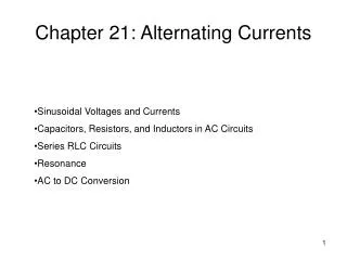
1.3c Current ElectricityAlternating Currents Breithaupt pages 74 to 79 November 14th, 2010
Direct and alternating current Direct current (d.c.) This is electric current that does not change direction in a circuit. Note: Direct current may change in size. Alternating current (a.c.) This is electric current that repeatedly reverses its direction. Phet AC & DC Circuit Construction Kit
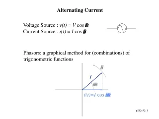
The sinusoidal variation of the voltage of the UK’s domestic mains supply. Sinusoidal voltage variation Sinusoidal voltage variation causes the most common type of alternating current. The frequencyof the voltage is equal to the number of complete cycles produced in one second. The UK’s a.c. supply has frequency of 50Hz. (USA is 60Hz) The peak value (V0 orI0) is the maximum current or pd in either direction. The UK’s a.c. voltage supply has a peak value of 325V. (USA is 155V)
The sinusoidal variation of the voltage of the UK’s domestic mains supply. The peak-to-peak value (2V0or2I0) is equal to the maximum variation in current or pd. With a pure a.c. this is equal to twice the peak value. The UK’s a.c. supply has a peak-to-peak voltage of 650V (2 x 325V) The period of the a.c. is the time taken to complete one cycle of variation. The UK’s a.c. supply has a period of 0.02s or 20ms.
The heating effect of a.c. The heating effect of current is independent of the direction of current flow. Power is the rate of heat transfer. With a resistor, R: P = I2 R With a varying current: P = < I2 > R Phet AC & DC Circuit Construction Kit
mean power power current With sinusoidal variation: < I2 > = ½ I02 And so: P = ½ I02 R
The root mean square (rms) value of an alternating current is equal to the value of direct current that would give the same heating effect as the alternating current in the same resistor. if: Irms2 R = ½ I02 R then: Irms2 = ½ I02 and so: Irms= I0/ √2 also with pds: Vrms= V0/ √2 and: P = Irms Vrms Root mean square values
Calculate the rms values of the UK and USA mains voltage supplies if the peak values, V0 are 325V and 155V respectively. Vrms= V0/ √2 UK: = 325V / √2 Vrms = 230V USA: = 155V / √2 Vrms = 110V Question
Complete: Answers: 3 8.49 2.83 24 325 6.5 1058 7.75 20 110 605 2 0.50 4 0.353 0.90 6 4.24 0.212
An oscilloscope (of traditional design) consists of a specially made electron tube and associated control circuits. • An electron gun at one end of the glass tube emits electrons in a beam towards a fluorescent screen at the other end of the tube. Light is emitted from the spot on the screen where the beam hits the screen. • The position of the spot on the screen is affected by the pd across either pair of deflecting plates (Y1Y2) and (X1X2). • The X-plates deflect the beam horizontally, the Y-plates vertically. In both cases the deflection of the beam is proportional to the applied pd.
cm squares The oscilloscope ‘graph’ scales Y-AXIS Potential difference Scale determined by the ‘Y-GAIN’ control Typical setting: 1V / cm + V 0V - V X-AXIS Time Scale determined by the ‘X-GAIN’ or ‘TIME-BASE’ control Typical setting: 0.1s / cm
Displaying a waveform1. The time base • The X-plates are connected to the oscilloscope’s time base circuit. • This makes the spot move across the screen, from left to right, at a constant speed. • Once the spot reaches the right hand side of the screen it is returned to the left hand side almost instantaneously. • The X-scale opposite is set so that the spot takes two milliseconds to move one centimetre to the right. (2 ms cm-1). NTNU Oscilloscope Simulation KT Oscilloscope Simulation
Displaying a waveform2. Y-sensitivity or Y-gain • The Y-plates are connected to the oscilloscope’s Y-input. • This input is usually amplified and when connected to the Y-plates it makes the spot move vertically up and down the screen. • The Y-sensitivity opposite is set so that the spot moves vertically by one centimetre for a pd of five volts (5 V cm-1). • The trace shown appears when an alternating pd of 16V peak-to-peak and period 7.2 ms is connected to the Y-input with the settings as shown. NTNU Oscilloscope Simulation KT Oscilloscope Simulation
Measuring d.c. potential difference All three diagrams below show the trace with the time base on and the Y-gain set at 2V cm-1. Diagram a shows the trace for pd = 0V. Diagram b shows the trace for pd = +4V Diagram c shows the trace for pd = -3V. NTNU Oscilloscope Simulation KT Oscilloscope Simulation
Measuring a.c. potential difference Let the time base setting be 10ms cm-1 and the Y-gain setting 2V cm-1. In this case the waveform performs one complete oscillation over a horizontal distance of 2 cm. Therefore the period of the waveform is 2 x 10ms period = 20 ms as frequency = 1 / period frequency = 1 / 0.020s = 50 Hz. The peak-to-peak displacement of the waveform is about 5cm. Therefore the peak-to-peak pd is 5 x 2V Peak-to-peak pd = 10V NTNU Oscilloscope Simulation KT Oscilloscope Simulation
Measuring a time interval The diagram opposite shows how an oscilloscope could be used to measure the speed of a pulse of ultrasound. A trigger pulse is sent from the oscilloscope to the transmitter. At the same time the spot is moved across the screen by the time base. When the receiver, which is connected to the Y-input, detects the pulse a deflection appears on the screen. If the time base had been set to 2 ms cm-1 then this pulse is shown to have taken about 7 ms to traverse the gap between the transmitter and receiver. Note: The time taken for the pulse to travel as an electric current in the wires is usually so small (< 1 microsecond) that it can be ignored.
Question 1 Measure the approximate period, frequency and peak-to-peak pd of the trace opposite if: Time base = 5ms cm-1 Y-gain = 5V cm-1 period = 50ms / 6 ≈8.7ms frequency ≈115 Hz peak-to-peak pd ≈20V
Question 2 Measure the approximate period, frequency and peak pd of the trace opposite if: Time base = 2ms cm-1 Y-gain = 0.5V cm-1 period = 20ms / 12 ≈1.7ms frequency ≈600 Hz peak pd ≈1.3V
Question 3 The trace shows how a waveform of frequency 286 Hz and peak-to-peak pd 6.4V is displayed. Suggest the settings of the time base and Y-gain amplifier. The period of a wave of frequency 286Hz = 1/285 = 0.0035s = 3.5ms One complete oscillation of the trace occupies 7cm. Therefore time base setting is 3.5ms / 7cm ≈0.5 ms cm-1 The peak-to-peak displacement of the trace is about 3.7 cm. Therefore the Y-gain setting is 6.4V / 3.7cm ≈2V cm-1
Internet Links • Oscilloscope - basic display function - NTNU • Oscilloscope Simulation - by KT • Lissajous figures - Explore Science • Lissajous figures- by KT
Core Notes from Breithaupt pages 74 to 79 • Explain what is meant by alternating current • Draw figure 1 on page 74 and define what is meant in the context of a.c. (a) peak value and (b) peak-to-peak value. • Explain what is meant by the r.m.s value of a sinusoidal current and voltage. State the equations relating r.m.s. values to peak values. • Calculate the rms values of the UK and USA mains voltage supplies if the peak values, V0 are 325V and 155V respectively. • Explain how an oscilloscope is able to display an alternating waveform. Your description should include an account of the role of the time base and the Y-sensitivity controls. • Explain how an oscilloscope can be used to measure: (a) d.c. voltage; (b) a.c. voltage; (c) a time interval & (d) frequency.
6.1 Alternating current and powerNotes from Breithaupt pages 74 to 76 • Explain what is meant by alternating current • Draw figure 1 on page 74 and define what is meant in the context of a.c. (a) peak value and (b) peak-to-peak value. • Explain what is meant by the r.m.s value of a sinusoidal current and voltage. State the equations relating r.m.s. values to peak values. • Calculate the rms values of the UK and USA mains voltage supplies if the peak values, V0 are 325V and 155V respectively. • Try the summary questions on page 76
6.2 Using an oscilloscopeNotes from Breithaupt pages 77 to 79 • Explain how an oscilloscope is able to display an alternating waveform. Your description should include an account of the role of the time base and the Y-sensitivity controls. • Explain how an oscilloscope can be used to measure: (a) d.c. voltage; (b) a.c. voltage; (c) a time interval & (d) frequency. • An oscilloscope is set with its time base on 10 ms cm-1 and Y-gain on 2V cm-1. Draw diagrams of the traces that would be displayed with inputs of: (a) 0V d.c.; (b) +5V d.c.; (c) – 3V d.c.; (d) sinusoidal a.c. of frequency 50Hz and peak value 4V. • Describe how an oscilloscope could be used to measure the speed of an ultrasound pulse. • Try the summary questions on page 79