Statistical Power
Statistical Power. H o : Treatments A and B the same H A : Treatments A and B different. Critical value at alpha=0.05. Points on this side, only 5% chance from distribution A. Frequency. A. Area = 5%. A could be control treatment B could be manipulated treatment.

Statistical Power
E N D
Presentation Transcript
Ho : Treatments A and B the same HA: Treatments A and B different
Critical value at alpha=0.05 Points on this side, only 5% chance from distribution A. Frequency A Area = 5% A could be control treatment B could be manipulated treatment
If null hypothesis true, A and B are identical Probability that any value of B is significantly different than A = 5% A B Probability that any value of B will be not significantly different from A = 95%
If null hypothesis true, A and B are identical Probability that any value of B is significantly different than A = 5% = likelihood of type 1 error A B Probability that any value of B will be not significantly different from A = 95%
What you say: Reality
If null hypothesis false, two distributions are different Probability that any value of B is significantly different than A = 1- beta = power A B Probability that any value of B will be not significantly different from A = beta = likelihood of type 2 error
Effect size A B Effect size = difference in means SD
1. Power increases as effect size increases Power Effect size A B Beta = likelihood of type 2 error
2. Power increases as alpha increases Power A B Beta = likelihood of type 2 error
3. Power increases as sample size increases High n A B
Alpha Effect size Power Sample size
Types of power analysis: A priori: Useful for setting up a large experiment with some pilot data Posteriori: Useful for deciding how powerful your conclusion is (definitely? Or possibly). In manuscript writing, peer reviews, etc.
Example : Fox hunting in the UK (posteriori)
Hunt banned (one year only) in 2001 because of foot-and-mouth disease. • Can examine whether the fox population increased in areas where it used to be hunted (in this year). • Baker et al. found no effect (p=0.474, alpha=0.05, n=157), but Aebischer et al. raised questions about power. Baker et al. 2002. Nature 419: 34 Aebischer et al. 2003. Nature 423: 400
157 plots where the fox population monitored. Alpha = 0.05 Effect size if hunting affected fox populations: 13%
157 plots where the fox population monitored. Alpha = 0.05 Effect size if hunting affected fox populations: 13% Power = 0.95 !
Class exercise: Means and SD of parasite load (p>0.05): Daphnia magna 5.9 ± 2 (n = 3) Daphnia pulex 4.9 ± 2 (n = 3) (1) Did the researcher have “enough” power (>0.80)? (2) Suggest a better sample size. (3) Why is n=3 rarely adequate as a sample size?
How many samples? PCBs in salmon from Burrard inlet and AlaskaIn an initial survey (3 individuals each), we find the following information (mean, standard deviation) Burrard – 120.5 ± 75.9 ppb Alaska – 75.2 ± 71.9 ppb The two error bars overlap, but that’s still a big difference and we only took 3 samples The difference could be “hidden” the sizes of the errors This would be reduced by increased samples, but how many should we take?
How many samples? Our difference between (q) is ~40, therefore if our confidence limits (SE) were <20ppb, we should have adifference between populations, Burrard – 120.5 ± 75.9 ppb Alaska – 75.2 ± 71.9 ppb How many samples do we therefore need??
Re-arrange the equation… So we should take 56 samples to be reasonably sure of a significant difference