Molecular Modeling and Informatics
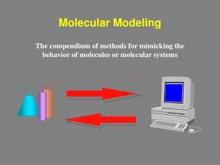
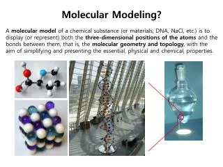
Molecular Modeling and Informatics. C371 Introduction to Cheminformatics Kelsey Forsythe. Characteristics of Molecular Modeling. Representing behavior of molecular systems Visual (tinker toys – LCDs) rendering of molecules

Molecular Modeling and Informatics
E N D
Presentation Transcript
Molecular Modeling and Informatics C371 Introduction to Cheminformatics Kelsey Forsythe
Characteristics of Molecular Modeling • Representing behavior of molecular systems • Visual (tinker toys – LCDs) rendering of molecules • Mathematical rendering (differential equations, matrix algebra) of molecular interactions • Time dependent and time independent realms
Molecular Modeling Valence Bond Theory + = Underlying equations: empirical (approximate, soluble) -Morse Potential ab initio (exact, insoluble (less hydrogen atom)) -Schrodinger Wave Equation
Empirical Models • Simple/Elegant? • Intuitive?-Vibrations ( ) • Major Drawbacks: • Does not include quantum mechanical effects • No information about bonding (re) • Not generic (organic inorganic) • Informatics • Interface between parameter data sets and systems of interest • Teaching computers to develop new potentials from existing math templates
MMFF Potential • E = Ebond+ Eangle+ Eangle-bond+ Etorsion+ EVDW+ Eelectrostatic
Atomistic Model History • Atomic Spectra • Balmer (1885) • Plum-Pudding Model • J. J. Thomson (circa 1900) • Quantization • Planck (circa 1905) • Planetary Model • Neils Bohr (circa 1913) • Wave-Particle Duality • DeBroglie (circa 1924) • Schrodinger Wave Equation • Erwin Schrodinger and Werner Heisenberg
Trajectory Real numbers Deterministic (“The value is ___”) Variables Continuous energy spectrum Wavefunction Complex (Real and Imaginary components) Probabilistic (“The average value is __ ” Operators Discrete/Quantized energy Tunneling Zero-point energy Classical vs. Quantum
Schrodinger’s Equation • - Hamiltonian operator • Gravity?
Hydrogen Molecule Hamiltonian • Born-Oppenheimer Approximation • Now Solve Electronic Problem
Electronic Schrodinger Equation • Solutions: • , the basis set, are of a known form • Need to determine coefficients (cm) • Wavefunctions gives probability of finding electrons in space (e. g. s,p,d and f orbitals) • Molecular orbitals are formed by linear combinations of electronic orbitals (LCAO)
Hydrogen Molecule • HOMO • LUMO
Hydrogen Molecule • Bond Density
Ab Initio/DFT • Complete Description! • Generic! • Major Drawbacks: • Mathematics can be cumbersome • Exact solution only for hydrogen • Informatics • Approximate solution time and storage intensive • Acquisition, manipulation and dissemination problems
Approximate Methods • SCF (Self Consistent Field) Method (a.ka. Mean Field or Hartree Fock) • Pick single electron and average influence of remaining electrons as a single force field (V0 external) • Then solve Schrodinger equation for single electron in presence of field (e.g. H-atom problem with extra force field) • Perform for all electrons in system • Combine to give system wavefunction and energy (E) • Repeat to error tolerance (Ei+1-Ei)
Correcting Approximations • Accounting for Electron Correlations • DFT(Density Functional Theory) • Moller-Plesset (Perturbation Theory) • Configuration Interaction (Coupling single electron problems)
Geometry Optimization • First Derivative is Zero • As N increases so does dimensionality/complexity/beauty/difficulty • Multi-dimensional (macromolecules, proteins) • Conjugate gradient methods • Monte Carlo methods
Modeling Programs • Observables • Equilibrium bond lengths and angles • Vibrational frequencies, UV-VIS, NMR shifts • Solvent Effects (e.g. LogP) • Dipole moments, atomic charges • Electron density maps • Reaction energies
Comparison to Experiments • Electronic Schrodinger Equation gives bonding energies for non-vibrating molecules (nuclei fixed at equilibrium geometry) at 0K • Can estimate G= H - TS using frequencies • Eout NOT DHf! • Bond separation reactions (simplest 2-heavy atom components) provide path to heats of formation
Ab Initio Modeling Limits • Function of basis and method used • Accuracy • ~.02 angstroms • ~2-4 kcal • N • HF - 50-100 atoms • DFT - 500-1000 atoms
Semi-Empirical Methods • Neglect Inner Core Electrons • Neglect of Diatomic Differential Overlap (NDDO) • Atomic orbitals on two different atomic centers do not overlap • Reduces computation time dramatically
Energetics Monte Carlo Genetic Algorithms Maximum Entropy Methods Simulated Annealing Dynamics Finite Difference Monte Carlo Fourier Analysis Other Methods
Large Scale Modeling (>1000 atoms) • Challenges • Many bodies (Avogardo’s number!!) • Multi-faceted interactions (heterogeneous, solute-solvent, long and short range interactions, multiple time-scales) • Informatics • Split problem into set of smaller problems (e.g. grid analysis-popular in engineering) • Periodic boundary conditions • Connection tables
Large Scale Modeling • Hybrid Methods • Different Spatial Realms • Treat part of system (Ex. Solvent) as classical point particles and remainder (Ex. Solute) as quantum particles • Different Time Domains • Vibrations (pico-femto) vs. sliding (micro) • Classical (Newton’s 2nd Law) vs. Quantum (TDSE)
Reference Materials • Journal of Molecular Graphics and Modeling • Journal of Molecular Modelling • Journal of Chemical Physics • THEOCHEM • Molecular Graphics and Modelling Society • NIH Center for Molecular Modeling • “Quantum Mechanics” by McQuarrie • “Computer Simulations of Liquids” by Allen and Tildesley
Modeling Programs • Spartan (www.wavefun.com) • MacroModel (www.schrodinger.com) • Sybyl (www.tripos.com) • Gaussian (www.gaussian.com) • Jaguar (www.schrodinger.com) • Cerius2 and Insight II (www.accelrys.com) • Quanta • CharMM • GAMESS • PCModel • Amber
Summary Types of Models • Tinker Toys • Empirical/Classical (Newtonian Physics) • Quantal (Schrodinger Equation) • Semi-empirical • Informatic Modeling • Conformational searching (QSAR, ComFA) • Generating new potentials • Quantum Informatics
Next Time • QSAR (Read Chapter 4)
MMFF Energy • Stretching
MMFF Energy • Bending
MMFF Energy • Stretch-Bend Interactions
MMFF Energy • Torsion (4-atom bending)
MMFF Energy • Analogous to Lennard-Jones 6-12 potential • London Dispersion Forces • Van der Waals Repulsions
Intermolecular/atomic models • General form: • Lennard-Jones Van derWaals repulsion London Attraction
MMFF Energy • Electrostatics (ionic compounds) • D – Dielectric Constant • d - electrostatic buffering constant