climate prediction
470 likes | 509 Vues
Dive into the science of climate change with insights on global warming trends, historical data, projected impacts, and effective climate modeling techniques. Learn about the complex dynamics of weather, climate, greenhouse gases, and the Earth's atmospheric system. Understand the significant role of human activities in influencing the climate and explore ways to predict and mitigate climate risks effectively. Discover how CPU power can aid in global climate prediction for a sustainable future.

climate prediction
E N D
Presentation Transcript
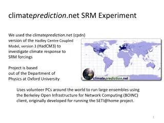
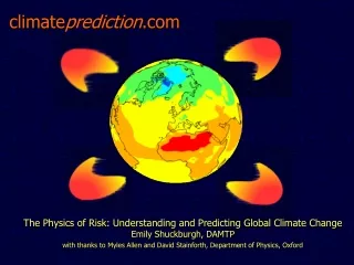
climateprediction.com The Physics of Risk: Understanding and Predicting Global Climate ChangeEmily Shuckburgh, DAMTP with thanks to Myles Allen and David Stainforth, Department of Physics, Oxford
The World’s climate in danger • “There is new and stronger evidence that most of the warming observed over the last 50 years is attributable to human activities” • “Human influences will continue to change atmospheric composition throughout the 21st century” • “The globally averaged surface temperature is projected to increase by 1.4 to 5.8° C by 2100” • The projected warming is very likely to be without precedent during at least the last 10, 000 years” Executive summary: Monday January 22, 2001
“A collective picture of a warming world” • Over the 20th century: • global-average surfacetemperature has increased (0.6° C) • temperature in lowest 8km increased in past 4 decades • global-average sea level has risen (0.1- 0.2 m) • snow & ice extent decreased - widespread retreat of glaciers • precipitation has increased (up to 1% per decade) • In Northern hemisphere increase in temperature in C20th likely to have been largest of any century, 1990s the warmest decade & 1998 the warmest year during past 1000 years. • Since 1750 there has been an increase of: • CO2(31%), CH4(151%) and N2O (17%) • present CO2 likely not exceeded in past 20, 000 years
The science of climate change • How can we model weather and climate? • How can we predict climate when we can’t predict next week’s weather? • What are the main uncertainties in climate prediction? • Quantifying risk: the science of probabilistic climate forecasting. • Harnessing idle CPU on YOURcomputer for global climate prediction.
Weather and Climate • “Weather” - tropospheric events associated with atmospheric flows of few 100 m & few days or less • Weather phenomena - chaotic, but atmospheric data averaged over a month - more regular • But exists interannual variability • “Climate” - state of the atmosphere averaged over several years +: the expected weather for a particular time of year. • It is determined by the boundary conditions of the atmosphere-ocean system: • solar irradiance (power output of the sun) • atmospheric composition (greenhouse gases...) • positions of continents, ice-sheets etc.
A simple climate model • Fs = 1375 W/m2, tube area pa2 • ~30% reflected away into space: albedo a = 0.3 • ~70% emitted as thermal infrared F0, from area 4pa2 • “effective temperature”, Te given by: sTe4=F0=¼Fs(1-a) 240 W/m2 • gives Te = 255K, lower than observed Ts = ~285K • why? - greenhouse effect Sun (energy input Fs) Earth (black body)
Solar and thermal radiation F0 Atmosphere: More solar radiation transmittedtsthan thermal radiation tt Atmosphere (Ta) Fg Earth (Tg) Fg=F0(1+ts)/(1+tt) 1.6 F0 =sTg4 Tg 286 K For doubled CO2, net radiation to space is reduced from ~240W/m2 by ~4W/m2 Climate system adjusts to restore balance.
Change in outgoing fluxes on 1K tropospheric warming • Direct emission: 4sTe3more energy to space • Warm moist air increases IR opacity: less energy emitted • Snow & ice melt: less energy reflected • Cloud amount and properties change • Net feedback factor: l = ~1.5W/m2/K
History of numerical modelling • Lewis Fry Richardson (Kings, Nat. Sci., 1900) • Whilst working as an ambulanceman in WW1 he produced the first numerical weather forecast, using a slide-rule. • During intervals between transporting wounded soldiers back from the front he made a 6-hour forecast of pressure and wind, starting from analysis of the conditions at 7am on 20 May 1910. • It took at least 6 months and was very inaccurate. • Proposed a “forecast factory” with some 26, 000 accountants • 25 years later Jule Charney formulated equations to be solved on a computer • First successful numerical prediction of weather in April 1950 using ENIAC computer
What is a climate model? • Dynamical equations + parameterisations
Dynamical equations • Newton’s 2nd law in horizontal(forces: pressure gradient and Coriolis) • Hydrostatic equation(gravity and pressure gradient) • Thermodynamic equation(temperature can change by “advection” or evapouration/condensation) • Continuity equation(conservation of mass) • Equation of State(perfect gas) • Water Vapour equation(amount of water vapour)
NWP parameterisations • Radiation • Surface and Sub-surface processes • Large-scale cloud and precipitation • Convection and convective precipitation • Gravity wave drag
Ocean-Atmosphere GCMs For climate modelling, physical processes not important for weather modelling must be included, in particular a representation of oceanic heat transfer
Evidence of “climate control”? Response to anthropogenic, solar and volcanic forcing
And how fast? • Surface oceans warm faster than depths. • Most initial warming occurs in top ~100m. • More sensitive climates (higher DT2xCO2) respond slower. • Ocean continues to adjust for centuries after atmospheric composition stabilises.
Climate model predictions: I Change In Near Surface Temperatures by the 2040s
Climate model predictions: II Predicted change at model resolution
How uncertain are these model predictions? • Models depend on “parameterisations” of processes too small to resolve. • Parameterisations represent the feedbacks between smaller and larger scales. • Many prescribed “parameters” (e.g. “ice fall speed in clouds”) are poorly constrained. • What is the impact of different parameter choices on model predictions? • Harder question: impact of model structure.
But climate is more than DTs • Simple re-scaling of model predictions only works for very large-scale variables. • Better approach: vary parameters within models and repeat the forecast. • But how much to vary parameters? • The Monte Carlo solution: • Vary parameters over very wide ranges • Simulate 1950-2050 changes with many models • Down-weight predictions from runs that fail to fit observed changes over 1950-2000
How many simulations? • The problem of non-linearity: you can’t just add up responses to different perturbations. • All combinations and permutations need to be tried, at least in principle. • 5 settings each of 9 parameters gives 59 permutations, or 2M simulations. • Current typical ensemble sizes with a comprehensive climate model: 4. • An impossible task?
Climateprediction.com • Most computing power is now on desks or in bedrooms, not supercomputing centres. • 100-year simulation with HadCM3L would take 8 months on an up-to-date PC. • Over 2M people have participated in SETI@home… • So we plan to: • Distribute ~2M versions of HadCM3L set up for… • Pre-packaged (unique) simulation of 1950-2050 • Estimate uncertainty from collated results
Participants will be able to: • Run up to 110 years of the UM. • View model output. • Compare their results on the web. • Run and view results from simplified models. • Run impact models?
Viewing model diagnostics Surface Temperatures
IS92a, GISS, 2050 Large cost (21) (6) (20) (11) (9) No cost (90) (16) (3) (4) (10) Large benefit (7) Impacts on Water
The participants? • To date we have:> 17,000 people > 45,000 PCs • Aiming for ~ 2 million PCs. • Who are they?IndividualsSmall businessesSchoolsLarge businesses ?
How many is “enough”? • There are many more than 9 underdetermined parameters in the model. • We cannot screen all possible combinations. • We can be more efficient by: • Screening parameter combinations first with a simplified model (same atmosphere, slab ocean). • Using intelligent sampling techniques (e.g. “genetic” algorithms). • We apply a range of future emissions scenarios to the most realistic models.
What of the real world? • Should we expect climate change in the real world to lie inside the range of predictions? • It depends on the quantity of interest: • Has the ensemble converged, or does perturbing more parameters change the estimated range? • Is the ensemble consistent with observations in this quantity? • Do we expect this variable to be well-simulated? • Basic problem: a probabilistic forecast cannot be tested with a single event -- the world can always surprise us.
Project Plan • UGAMP / researchers release. Soon • Single parameter sensitivity tests with the slab model. • Linux release. Year End • Multiple parameter perturbations with the slab model. • Initial condition ensemble. • Main windows release. Next year • Casino-21: A physics ensemble experiment.
climateprediction.com www.climateprediction.com