Download
1 / 34
340 likes | 527 Vues
Physiology-based modeling and quantification of auditory evoked potentials. Cliff Kerr Complex Systems Group School of Physics, University of Sydney. Introduction. Aim: to develop a physiology-based method of evoked potential (EP) analysis, in order to: Provide a means to quantify EPs

E N D
Physiology-based modeling and quantification of auditory evoked potentials Cliff Kerr Complex Systems Group School of Physics, University of Sydney
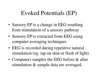
Introduction • Aim: to develop a physiology-based method of evoked potential (EP) analysis, in order to: • Provide a means to quantify EPs • Relate EP data to brain physiology • Implementation: biophysical modeling and deconvolution of EEG data
Outline • What are evoked potentials? • Fitting: • Methods: theory, data, implementation • Results: group average waveforms • Application: arousal • Deconvolution: • Motivation • Theory • Results: synthetic and experimental data • Discussion and summary • Challenges and future directions
EEG: EP: Time-locked averaging V(mV) V(mV) t(s) t(s) What are EPs? stimulus:
Traditional analysis: scoring Standard Target N1 6.5 mV 112 ms P50 1.2 mV 56 ms N1 8.0 mV 120 ms N2 3.4 mV 224 ms P2 -8.0 mV 264 ms P3 -19.6 mV 320 ms
Theory e Cortex i r Thalamus s Brain stem n
Theory • Physiology-based continuum modeling: uses 11 vs. 1,000,000,000,000,000 connections • Five populations of neurons: • Sensory (excitatory; labeled n) • Cortical (excitatory & inhibitory; e & i) • Thalamic relay (excitatory; s) • Thalamic reticular (inhibitory; r) • Five neuronal loops: • cortical (Gee, Gei ) • thalamic (Gsrs) • thalamocortical (Gese , Gesre) e i r s n
Theory • Model has 14 parameters: • 5 for neuronal coupling strength (Gee, Gei , Gese , Gesre , Gsrs ) • 4 for neuronal network properties (a, b, g, t0) • 5 for stimulus properties (tos, ts, ros, rs) • Most important parameters are the gains Gab (coupling strength between neuron populations) • Model describes conversion process (auditory stimulus → neuronal activity → scalp electrical field) using an analytic transfer function fe/fn:
Theory • Direct impulse: • Cortical modulation: • Corticothalamic modulation: • Transfer function:
Theory • Impulse: • Time-domain impulse response:
Data • Sampled from 1527 normal subjects: • Aged 6-80 years • Equal numbers male & female • No neurological diseases, chemical dependencies, etc. • Stimulus: 1 tone/second for 6 minutes (280 standard tones, 80 target tones) • Used to produce group average standard and target EPs (generated using >100,000 single trials!)
c2 P2 P1 Fitting 1) Initial parameters are chosen .
2) Gradient descent algorithm reduces c2 of fit c2 P2 P1 Fitting .
3) Process is repeated using different initialisations c2 P2 P1 Fitting
Results • Excellent fits to standards (up to 400 ms)
Results • Excellent fits to targets (up to 300 ms)
Results • Possible changes in neuronal network properties:
Results • Probable changes in neuronal coupling strengths:
Results • Definite changes in stability parameters:
0 2 4 6 -5 μV 0.1 s Application: arousal • Same task (auditory oddball) • 43 subjects • Averaged over ten time intervals of 40 seconds each task duration (min)
Application: arousal • Increased cortical activity → decreased acetylcholine?
Deconvolution: motivation • In model, thalamocortical loop → N2 feature of targets • Could target response = standard response + delayed standard response?
Theory • Assumption: responses are product of task-dynamic and task-invariant properties: • Fourier transform: • Take the ratio of the two: • Inverse Fourier transform to get the result:
Theory • Direct deconvolution is uselessly noisy: • Hence, use Wiener deconvolution:
Discussion and summary • Physiology-based EP fitting can be achieved • Offers significant advantages over traditional methods • Results tentatively suggest physiology underlying stimulus perception: • Increase in stability: required for a transient response • Arousal determined by thalamocortical activity: standards show increased inhibition, targets show increased excitation • Standards generated by ≈1 thalamocortical impulse, targets by ≈2
Challenges • Fitting challenges • Degeneracy • Constraints • Testability • Deconvolution challenges • Noise and artifact • What are we looking for? • Physiological challenges • Only 1D information • What’s signal?
Future directions • How does the brain change with age? Standard Target
Future directions • Can our model account for depression?
Future directions • Modeling the ERP “zoo” • modality • arousal • disease • drugs Visual: Somatosensory: Oddball: Quiet sleep: Bipolar: Radiculopathy: Carbonyl sulfide: Ecstasy:
Acknowledgements Chris J. Rennie Peter A. Robinson Jonathon M. Clearwater Andrew H. Kemp Brain Resource Ltd.