Pressure Concepts
Pressure Concepts. Petroforma - Luanda . Balancing Formation Fluid Pressures. Overbalance: Mud pressure in excess of pressure on pore fluids Controlled by fluid density and/or column height; required condition for conventional drilling Underbalance:

Pressure Concepts
E N D
Presentation Transcript
Pressure Concepts Petroforma - Luanda
Balancing Formation Fluid Pressures Overbalance: Mud pressure in excess of pressure on pore fluids Controlled by fluid density and/or column height;required condition for conventional drilling Underbalance: Mud pressure less than pressure on pore fluids
Primary well control is the process of maintaining an effective hydrostatic pressure above formation pressure but less than the formation breakdown pressure. Maintaining Primary Well Control In most rotary drilling operations, an important objective is to maintain a state of primary well control.
If primary well control is lost, a kick (unwanted intrusion of fluids into the wellbore) may occur. A kick can turn into an uncontrolled blowout. In such a case, secondary well control measures come into effect. This primarily involves the use of surface well control equipment. Loss of Primary Well Control
Different Expressions of Pressure 1. As direct measurement in different units (psi, bar, kg/cm2, etc.) 2. EMD (Equivalent mud density) 3. Gradient (psi/ft, kg/cm2 per 10 m) 4. Potential
A pressure is a force divided by the surface upon which this force applies. Pressure Pascal = Force Newton / Surface m2 The official pressure unit is the Pascal It is a very small unit: 1 Pascal = 1 Newton/m2 1 bar = 105 Pascal 1 atm = 1,013 *105 Pascal A practical unit on the rig is the kgf/cm2: 1 kgf/cm2 =0.981 bar In API, the unit is the pound per square inch (psi): 1 bar = 14.4988 psi
Exercise 1 – Unit Conversions 1 kgf/cm2 =0.981 bar 1 bar = 14.4988 psi Convert the following values to the requested units: 25 kgf/cm2 = bars 15 Bars = psi 155 Psi = bars 24.53 217.48 10.69
Hydrostatic Pressure • Hydrostatic Pressure is the pressure exerted by the weight of a static column of fluid. • Function of: • - Height of the column • - Fluid density only. The geometry and dimensions of the fluid column have no effect on hydrostatic pressure.
Pascal’s Demonstration The scientistPascal bet he could destroy a barrel with just a pint of water: He fixed a long and thin tube on the barrel and poured in the water. Despite the tiny volume of the water, the height was enough to make the barrel explode*! *Also credited to the Flemish sicentist Simon Stevinus
Hydrostatic Pressure Formula: Ph= d * g * H With Ph = hydrostatic pressure (Pascal) d = Fluid specific gravity (kg/m3) H = Vertical height of fluid (m)
Metric units: H*d 10 Where: Ph= hydrostatic pressure ( kg/cm2) d = Fluid specific gravity (kg/l) H = Vertical height of fluid (m) NB : you must use 10.2 with pressure in bars Ph = Hydrostatic Pressure Formula API units: Ph = 0.052*H*d Where: Ph = hydrostatic pressure (psi) d = Fluid density (ppg) H = Vertical height of fluid (ft)
Metric units: H*d 10 Ph = Exercise 2 – Hydrostatic Pressure API units: Ph = 0.052*H*d • Calculate Ph in the following examples: • Height of fluid (m): 1000 Fluid density (kg/l): 1.5 Ph (kgf/cm2): • Height of fluid (ft): 5000 Fluid density (ppg): 10 Ph psi: 150 2600
Pipe Annulus Pipe Annulus Weighted Mud The ‘U-tube’ Effect If the mud weights in the pipes and annulus are different, a ‘U-tube’ effect occurs due to the difference of Ph, as the system seeks equilibrium. The slug of weighted mud pumped just prior to a trip takes advantage of this effect to keep the inside of the pipe dry at drill floor level.
Pf &Ph (due to MW) in kgf/cm2 Depth (m) 1.30 1.20 1.03 Pressure vs. Depth Plot The pressure vs. depth plot provides a convenient means to show changes in pressure gradient with depth.
Pressure vs. Depth Plot Pressure from RFT (kgf/cm2) Another purpose of this type of plot is to determine the contacts between fluids in a reservoir by tracing the trend lines of the RFT pressure data. Gas/oil contact (m) Oil/water contact (m) Depth (m)
Pressure vs. Depth Plot The pressure vs. depth plot also allows easy comparison of pressure parameters whose interaction may result in drilling problems, such as formation pressure and fracture gradient.
Formation (Pore) Pressure Formation pressure is the pressure of the fluid contained in the pore spaces of the sediments. Pressure 0 Negative pressure anomaly Pressure less than hydrostatic pressure. Hydrostatic zone Pressure remains in normal hydrostatic regime. Positive pressure anomaly Pressure more than hydrostatic pressure. Usually limited by overburden stress. Overburden pressure d = 2.31 Hydrostatic pressure d = 1.08 D e p t h Hydrostatic pressure d = 1.00 Normal pressure regime Negative pressure anomaly Positive pressure anomaly 5000 0 500 1000 1500
Equivalent Mud Weight (EMW) Depending on drilling conditions, the equivalent mud weight may be greater or less than the actual mud weight. Equivalent MW < actual MW Mud losses Swabbing Fluid Influx (kick) Equivalent MW > actual MW Leak Off Test/Formation Integrity Test Surge Circulation (Hydrostatic + annular pressure loss)
Equilibrium Mud Weight Well - A Depth 0 m EMW for well No 1 = 1 SG (200 X 10) / 2000 (Mud weight required to balance formation pressure) Well - B Depth 1000 m EMW for well No 2 = 2 SG (200 X 10) / 1000 (Mud weight required to balance formation pressure ) Fm. Press. 200 kgf/cm2 Depth 2000m Knowledge that the formation pressure is 200 is not enough. We have to see it in relation to the balancing mud column.
Static Circulating Equivalent Circulating Density (ECD) This is the effective density of the circulating fluid when pressuredrop in the annulus is considered: Ph + annular pressure loss, converted to mud weight ECD thus implies that the pressure at any point in the annulus while circulating will be higher than when the fluid is at rest (static). Metric: ECD = ((Ph + APL in kg/cm2)X 10) / Depth in m API: ECD = ((Ph + APL in psi) / Depth in ft) / .052
Swab:a decrease of effective hydrostatic caused by mechanical movement upwards Surge:an increase of effective hydrostatic caused by mechanical movement downwards Swab/Surge The drill string can act like a piston when moved vertically, and this movement can affect the wellbore pressure.
Swab/Surge Excessive swabbing, for example by pulling the pipe too fast during a trip out of the hole, can result in a kick. Excessive surge, usually from running in too fast, can result in formation breakdown and lost circulation. As these effects can be subtle, we must monitor trips carefully, by keeping a trip sheet and by observing the differential volume (volume +/-) parameter on the real-time data acquisition system.
Exercise 5 – Equivalent Mud Densities Calculate the EMW for the following cases: Well total depth (m) 2000Mud weight in hole (kg/l) 1.20 A. During a trip, the driller forgot to fill the hole and the mud level is lower than normal; its distance from flow line is 100m; EMW = kg/l 1.14 B. During a Leak Off Test, the pressure reached A maximum of 10 kgf/cm2; EMW = kg/l 1.25 C. Circulation starts; the pressure losses in the annulus is 4 kg/cm2; ECD = kg/l 1.22
GPf MW FRACS Pressure (kg/cm2) Depth (m) Plotting Pressure Gradients MW and pressure gradients may be plotted on the same graph, allowing a comparison between MW, Formation pressure gradient, Fracture gradient and Overburden gradient.
Overburden Stress: OVBP Name convention : • OVBP for overburden Pressure(often called S in the literature) • OVBg for local gradientFor intervals with constant density • OVBG for averaged Gradient, referenced to flow line,expressed in EMW.
Cumulative weight of rocks + fluid Overburden Stress: OVBP Overburden stress is the pressure exerted by the weight of the overlying sediments. The term pressure is usually applied for fluid hence the word stress. OVBP =P + s OVBP: Overburden Stress (total pressure) P: Pore Pressure s:Pressure supported by rock matrix (effective stress) Matrix: Rocks + Cement (Solids) Contribution to total weight will depend on matrix density. Fluid: Fluid assumed as water; gas will affect the density.
(overburden) S 1 S 2 S 3 Matrix Stress Components Unlike liquids, solids can withstand different loads in various directions: Imagine a cube of porous rock somewhere in the subsurface… We can divide the stresses into 3 resulting forces according to the 3 directions of space: S1 can be considered the Overburden, S2 and S3 the tectonic forces. Open hole ovalization can give an idea of the difference between S2 and S3.
S 1 S 2 S 3 Terzaghi and Peck Equation In a porous rock, the fluid may support part of the stress (due to undercompaction) and the total stress will have 2 components: OVBP = P + s(Terzaghi equation) With OVB = Total stress (kgf/cm2) P = Pore pressure ( or formation pressure) (kgf/cm2) s = Effective stress (on the grains of the rock) (kgf/cm2) Consequently: S1 = P + s1 (OVBP) S2 = P + s2 S3 = P + s3 So, in theory, the formation pressure is limited by the overburden!
Overburden Stress Formula Metric units: H*rb 10 Where: Ph = hydrostatic pressure (kg/cm2) rb = Average formation bulk density (no unit) H = Vertical thickness of overlying sediments (m) API units: OVBP = H*rb*0.433 Where: Ph = hydrostatic pressure (psi) rb = Average formation bulk density (no unit) H = Vertical thickness of overlying sediments (ft) OVBP =
Bulk Density Formula The bulk density of a sediment is a function of the matrix density, the porosity and the density of the fluid in the pores. rb = (f * rf) + (1-f) * rm • Where: • rb = Bulk density (no unit) rf = Formation fluid density (no unit)f = Porosity (from 0 to 1)rm = Matrix density (no unit)
Overburden Gradient Sediments laid down in the basin are buried deeper and deeper with the continuation of the sedimentary process. BURIAL INREASES THE OVERBURDEN INCREASE OF OVERBURDEN LEADS TO COMPACTION COMPACTION DECREASES POROSITY Porosity Clay / Shale behaviour Porosity decrease is rapid in the upper part of the curve - shallow depth and unconsolidated section. The curve levels off in compacted clay which progressively changes to claystone and shale. Sandstone For the sandstone compaction is due to realignment of grains and effects of diagenesis. Clay / Shale D e p t h Sandstone
Overburden Gradient • Overburden gradient is calculated by averaging density from surface to the depth of interest. • Knowledge of overburden gradient is necessary: • For evaluation of formation pressure • For calculation of fracture gradient • Bulk density increases with depth and also varies depending on fluid and lithology. Hence averaging is necessary. OVBG OVBG (API) (Metric)
Overburden Gradient Consider 3 layers of different densities: Interval Thickness app. density interval ovb M M rb ovb pressure gradient 0 - 100 100 2.1 21 2.1 100 - 200 100 2.3 23 2.2 200 - 400 200 2.5 50 2.35 Gr = Press x 10 / Int 1) 100 x 2.1 / 10 = 21 kg / cm2 (21) x 10 / 100 = 2.1 2) 100 x 2.3 / 10 = 23 kg / cm2 (21+23) x 10 / 200 = 2.2 3) 200 x 2.5 / 10 = 50 kg / cm2 (21+23+50) x 10 / 400 = 2.35
Overburden Gradient Example overburden density curves (Mouchet and Mitchell, 1989) Some literature quotes average bulk density as 2.31 kg/l, or 1 psi/ft This is an approximate value only. For accurate interpretation it is necessary to calculate actual values.
Density 2.31 Density 2.31 Sea Bed Depth Depth Onshore curve Offshore curve Overburden Gradient Offshore wells have a water column that affects bulk density. This effect can be very important in moderate- to deep-water areas Note the difference: Onshore overburden exceeds 2.31. Off-shore overburden remains below 2.31.
Estimating Fracture Gradient Why do we need to know the Fracture Gradient? • It is essential to increase mud weight during drilling of an abnormally pressured section. • There is a limit to which MW can be increased. • Shallower parts of the well are weaker than deeper, more compacted strata. • Weakest point in the well is just below casing. • Increase in MW beyond limit may open fractures, possibly leading to mud loss and kick. • Mud loss may also occur at the limit of the pressure in porous rocks such as SST and LST. • MW is also limited by the casing and BOP.
Fracture Gradient Fracture gradient is in part controlled by the overburden gradient. In general, the lower the overburden gradient, the lower the fracture gradient. In deepwater drilling, the range of usable mud densities may be very narrow due to the low fracture gradients involved. The ‘Waterdepther’ spreadsheet shows this relationship graphically. Note how increased water depth and/or formation pressure tends to increase the number of casing strings required.
Fracture Gradient In exploratory drilling, the limit or fracture gradient is determined by Leak-off Test (LOT) or Formation Integrity test (FIT). LOT/FIT results also help define: 1. Adjustments to Casing Program and MW 2. Maximum pressure permissible during kick control to avoid internal blow out. 3. Hydraulic fracture pressure required for stimulation. A LOT tests the formation to the fracture-opening pressure, while a FIT merely tests to a pre-determined value assumed to be slightly less than the maximum pressure allowable. FIT is preferred when formations are already known to be weak.
Pump… in a well with closed BOPs… until the pressure in the well reaches fracturation pressure of the formation. Leak-off Test It is usually performed after drilling a few meters below the last intermediate casing shoe. Normally, the cement pump is used, to better control the volume and pressure pumped.
LOT pressure C D E B Pressure Pumping A Volume l Time Leak-off Test A : Start Pumping AB : Elastic behaviour of formation. B : Leak off - fracture BC : Mud penetrates formation C : Pumping Stopped. CD : Fracture propagation ceases Pressure falls to a stabilised pressure (D) which is less than or equal to B E : Bleed-off. Mud recovered should be equal to the volume pumped. If less, the fractures remained open; pressure at D in this case will also be less than pressure at B.
FIT Pressure Bleed off Pressure Pump off Time Volume Formation Integrity Test
Calculating Maximum Allowable Mud Density First calculate bottom hole pressure: PFRAC = PLOT + Mud Hydrostatic Pressure in the well Then determine EMW: Metric: EMW = (Ph kg/cm2 X 10) / Depth in m API: EMW = (Ph psi / Depth in ft) / .052
Exercise 6 -- Fracture Gradient Calculate Fracture - LOT- EMW from the data given below. Drilled Depth: 1912 m. Casing shoe at 1900 m. MW: 1.2 SG LOT press.: 56 kg/cm2 Hydrostatic Pressure = LOT pressure = Total leak off pressure = Frac. EMW = 1900 X 1.2 / 10 = 228 kg/ cm2 56 kg/cm2 284 kg/cm2 284 X 10/1900 = 1.49