Download
1 / 26
310 likes | 585 Vues
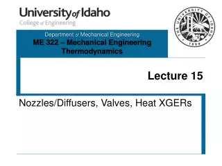
Lecture 15 Resistivity-GPR. Death Valley Basin. Furnace Creek Fault. Resistivity. SYSCAL R1 Plus – resistivity meter for medium-depth exploration can be used for: geological mapping groundwater exploration. Put 48 stainless steel electrodes in the ground every five meters

E N D
Resistivity • SYSCAL R1 Plus – resistivity meter for medium-depth exploration • can be used for: • geological mapping • groundwater exploration
Put 48 stainless steel electrodes in the ground every five meters Attach the electrodes to the cable with clips Press start on the box
resistance + - Battery current Ohm’s Law + - V I R
Resistivity Double length double R Double area halve R R proportional to length/area Area current length
Wenner Array Ohm’s law V=IR Apparent resistivity Voltage (V) Current (I) Resistance (R) a=2πa ΔV/I Electric Sounding Shallowest = a Deepest = spacing*(round down((number of electrodes -1) /3))
I V r1 r2 r3 r4 Theory
Mtlab Program for 2 Layer Resistivity %Resistivity function from Pages 529 Telford et al., Applied Geophysics %Second Edition clear f aarray=x; %meters rho1=a(1); rho2=a(2); z=a(3); k=(rho2-rho1)/(rho2+rho1); %Equation 8.38 for i=1:length(aarray); aa=aarray(i); m=1:10000; D=sum( k.^m./((1+(2*m*z./aa).^2).^0.5) )-sum( k.^m./((4+(2*m*z./aa).^2).^0.5) ); rhoa=rho1*(1+4*D); f(i)=rhoa; end figure(1) plot(log10(aarray),log10(f),log10(aarray), log10(y),'*')
Pseudosections Roughly how resistivity varies vertically and laterally Electrical imaging creates ‘true’ section using tomographic theory
Middle Mountain Resistivity • Two resistivity lines were laid out for Middle Mountain • The anomaly colored yellow is most likely the water table dammed by the faults • From the 1st line to the 2nd line the water table increases in size likely due to the increase in distance between the fault splays Line 1 Line 2
SAF Splay Map view Model to explain increase in size of water table