Download
1 / 49
490 likes | 528 Vues
Learn about the foundations of Signal Detection Theory in psychophysics, exploring if sensitivity is discrete or continuous, the role of noise, and how sensitivity and response bias interact. Discover key assumptions and statistical measures used to evaluate detection processes.

E N D
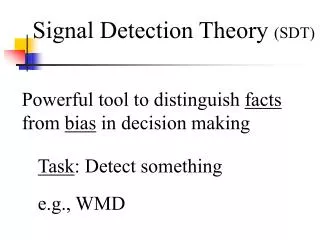
Origins of Signal Detection Theory • Problem in Psychophysics • Thresholds: is sensitivity discrete or continuous? • Sensitivity confounded with response bias
Thresholds • Solution: detection theory (engineering)
Signal Detection Theory Response Yes No Signal State of the World Noise
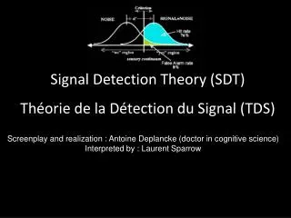
Assumptions of Signal Detection Theory • Noise is always present (i.e. in the nervous system and/or in the signal generating system) • The noise is normally distributed with σ2 = 1 • For Gaussian model • When a signal is added to the noise, the distribution is shifted upward along the sensory dimension. Variance remains constant (equal variance model).
Assumptions of Signal Detection Theory • Observers are both sensors and decision makers • To evaluate the occurrence of an event, observers adopt a decision criterion • Sensitivity and Response Bias are independent • Statistical • Theoretical • Empirical
Sensitivity d’ = zH - zF d’ Task Person >3.5 very easy very sensitive 2.6-3.5 moderately easy moderately sensitive 1.6-2.5 moderately difficult moderately insensitive <1.5 very difficult very insensitive
Relation of d’ to Other Statistics If μn=0 and σn=1 (i.e., if the N distribution is unit normal) then the ROC function, in its most general form, is
Response Bias Lenient: 0-1 Unbiased: 1 Conservative: 1- 8 = f(SN)/f(N) c = -.5(zH + zF) Lenient: <0 Unbiased: 0 Conservative: >0
Three values of 2 1 3 P(event|x) N SN Sensory magnitude (X)
ROC Curve in Z-score form 1 ZH 0 0 1 ZFA
ROC for σ2N = σ2SN 3 0 ZH -3 3 -3 0 ZFA
What is Independence? • Statistical: P(A|B)=P(A) PB|A)=P(B) • Theoretical/Logical: β can vary independently of d’ • Empirical: experimental evidence is consistent with the independence assumption (e.g. Form of empirical ROC)
Three values of 2 1 3 P(event|x) N SN Sensory magnitude (X)
ROC Curve in Z-score form 1 ZH 0 0 1 ZFA
ROC for σ2N = σ2SN 3 0 ZH -3 3 -3 0 ZFA
Alternative Sensitivity Measures Az: Area under the ROC (e.g., see Swets,1995, ch. 2-3; Swets & Pickett, 1982) Range: from .5—1.0 Underlying distributions can have unequal variances Assumes that the underlying distributions can be monotonically transformed to normality ZH= a + bZF
‘Non-parametric’ Measures: Sensitivity Not really non-parametric: No distribution assumed, but follows a logistic distribution (Macmillan & Creelman, 1990)
‘Non-parametric’ Measures: Response Bias For applications to vigilance, see See, Warm, Dember, & Howe (1997)
What if the Situation is More Complex? Response State of the World
Identification and Categorization 1 5 2 6 4 3 Response 6 5 4 2 3 1 7 x
Fuzzy Logic Traditional Set Theory: A ∩ A = 0 Fuzzy Set Theory: A ∩ Ā ≠ 0 One assigns non-binary membership, or degrees of membership, to classes of events (fuzzification).
Elements of Fuzzy Signal Detection Theory • Events can belong to the set “signal” (s) to a degree ranging from 0 to 1 • Events can belong to the set “response” (r) to a degree ranging from 0 to 1
Computation of FSDT Measures • Select mapping functions for signal & response dimensions • Assignment of degrees of membership to the four outcomes (H, M, FA, CR) using mixed implication functions. • Compute fuzzy Hit, Miss, False Alarm, and Correct Rejection Rates • Compute detection theory measures of sensitivity and response bias
2. Assignment of Set Membership to Categories • Mixed Implication Functions • H = min (s,r) • M = max (s-r, 0) • FA = max (r-s, 0) • CR = min (1-s, 1-r)
3. Computation of Fuzzy Hit and False Alarm Rate H= Σ(Hi)/ Σ(si) for i=1 to N M = Σ(Mi)/ Σ(si) for i =1 to N FA = Σ(FAi)/ Σ(1-si) for i=1to N CR = Σ(CRi)/ Σ(1-si) for i= 1 to N
Comparison of Fuzzy and Crisp ROC Curves Crisp Fuzzy
Comparison of Fuzzy and Crisp ROC Curves Crisp Fuzzy
Response Time as a Function of Degree of Stimulus Criticality 1100 1000 900 Response Time (msec) Transition 800 hh 700 hl 600 lh 500 ll 1 2 3 4 5 6 7 1 0 Stimuli
Reaction Time as a Function of Stimulus Value: 80 msec Discrimination
Reaction Time as a Function of Stimulus Value: 20 msec Discrimination