Key Principles of Statistical Inference

1. Key Principles of Statistical Inference

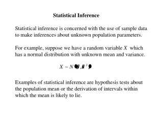
2. Statistical Inference • Involves obtaining information from sample of data about population from which sample was drawn & setting up a model to describe this population • When random sample is drawn from population, every member of population has equal chance of being selected in the sample

3. Types of Statistical Inference • Parameter Estimation takes two forms • Point Estimation: when estimate of population parameter is single number • Ex. Mean, median, variance & SD • Hypothesis-Testing: • More common type

4. Normal Curve

5. Normal Curve • 68% of cases fall within + 1 SD of the mean • 96% of cases fall within + 2 SD of the mean • 100% of cases fall within + 3 SD of the mean.

6. Normal Distribution & Z score • When variable’s mean & SD are known, any set of scores can be transformed into z-scores with • Mean = 0 SD = 1 • Two Important Z scores: • + 1.96z = 95% confidence interval • + 2.58z = 99% confidence interval

7. Percentiles • Tells the relative position of a given score • Allows us to compare scores on tests with different means & SDs. • Calculated as • (# of scores less than given score) X 100 total # of scores

8. Percentile • 25th percentile = 1st quartile • 50th percentile = 2nd quartile Also the median • 75th percentile = 3rd quartile

9. Standard Scores • Way of expressing a score in terms of its relative distance from the mean • z-score is example of standard score • Standard scores are used more often than percentiles • Transformed standard scores often called T-scores • Usually has M = 50 & SD = 10

10. Standard Error of Mean (SE) • Is standard deviation of the population • Constant relationship between SD of a distribution of sample means (SE), the SD of population from which samples were drawn & size of samples • As size of sample increases, size of error decreases • The greater the variability, the greater the error

11. Probability Axioms • Fall between 0% & 100% • No negative probabilities • Probability of an event is 100% less the probability of the opposite event

12. Definitions of Probability • Frequency Probability based on number of times an event occurred in a given sample (n) # of times event occurred X 100 total # of people in n • P ………………… Probability value that observed data are consistent with null hypothesis

13. Definitions of Probability • Subjective Probability:percentage expressing personal, subjective belief that event will occur • p values of .05, often used as a probability cutoff in hypothesis-testing to indicate something unusual happening in the distribution

14. Hypothesis-Testing • Prominent feature of quantitative research • Hypotheses originate from theory that underpins research • Two types of hypotheses: • Null Ho • Alternative

15. Null Hypothesis - Ho • Ho proposes no difference or relationship exists between the variables of interest • Foundation of the statistical test • When you statistically test an hypothesis, you assume that Ho correctly describes the state of affairs between the variables of interest

16. Null Hypothesis - Ho • If a statistically significant relationship is found (p < .05), Ho is rejected • If no statistically significant relationship is found (p. > .05), Ho is accepted

17. Alternative Hypothesis - Ha • A hypothesis that contradicts Ho • Can indicate the direction of the difference or relationship expected • Often called the research hypothesis & represented by Hr

18. Sampling Error • Inferences from samples to populations are always probabilistic, meaning we can never be certain our inference was correct • Drawing the wrong conclusion is called an error of inference, defined in terms of Ho as Type I and Type II

19. H0 True H0 False Accept H0 Right decision  = significance Wrong decision 1-b = type II error Reject H0 Wrong decision 1 -  = type I error Right decision B = power Types of Errors • We summarize these in a 2x2 box: Decision

20. Types of Errors • Type I error occurs when you reject a true Ho • Called alpha error • Type II error occurs when you accept a false Ho • Called beta error

21. Types of Errors • Inverse relationship between Type 1 & Type II errors. • Decreasing the likelihood of one type of error increases the likelihood of the other type error • This can be done by changing the significance level • Which type of error can be most tolerated in a particular study?

22. Significance Level • States risk of rejecting Ho when it is true • Commonly called p value • Ranges from 0.00 - 1.00 • Summarizes the evidence in the data about Ho • Small p value of .001 provides strong evidence against Ho, indicating that getting such a result might occur 1 out of 1,000 times

23. Testing a Statistical Hypothesis • State Ho • Choose appropriate statistic to test Ho • Define degree of risk of incorrectly concluding Ho is false when it is true • Calculate statistic from a set of randomly selected observations • Decide whether to accept or reject Ho based on sample statistic

24. Power of a Test • Probability of detecting a difference or relationship if such a difference or relationship really exists • Anything that decreases the probability of a Type II error increases power & vice versa • A more powerful test is one that is likely to reject Ho

25. One-Tailed & Two-Tailed Tests • Tails refer to ends of normal curve • When we hypothesize the direction of the difference or relationship, we state in what tail of the distribution we expect to find the difference or relationship • One-tailed test is more powerful & is used when we have a directional hypothesis

26. Tailedness Significantly different from mean Significantly different from mean .025 .025 Tail Tail Two-Tailed Test- .05 Level of Significance Significantly different from mean .05 One-Tailed Test- .05 Level of Significance

27. Degrees of Freedom (df) • The freedom of a score’s value to vary given what is known about other & the sum of the scores • Ex. Given three scores, we have 3 df, one for each independent item. Once you know mean, we lose one df • df = n - 1, the number of items in set less 1 • Df (degrees of freedom): the extent to which values are free to vary in a given specific number of subjects and a total score

28. Confidence Interval (CI) • Degree of confidence, expressed as a percent, that the interval contains the population mean (or proportion), & for which we have an estimate calculated from sample data • 95% CI = X + 1.96 (standard error) • 99% CI = X + 2.58 (standard error)

29. Relationship Between Confidence Interval & Significance Levels • 95% CI contains all the (Ho) values for which p > .05 • Makes it possible to uncover inconsistencies in research reports • A value for Ho within the 95% CI should have a p value > .05, & one outside of the 95% CI should have a p value less than .05

30. Statistical Significance VSMeaningful Significance • Common mistake is to confuse statistical significance with substantive meaningfulness • Statistically significant result simply means that if Ho were true, the observed results would be very unusual • With N > 100, even tiny relationships/differences are statistically significant

31. Statistical Significance VSMeaningful Significance • Statistically significant results say nothing about clinical importance or meaningful significance of results • Researcher must always determine if statistically significant results are substantively meaningful. • Refrain from statistical “sanctification” of data

32. Sample Size Determination • Likelihood of rejecting Ho (ie, avoiding a Type II error • Depends on • Significance Level: P value, usually .05 • Power: 1 - beta error, usually set at .80 • Effect Size: degree to which Ho is false (ie, the size of the effect of independent variable on dependent variable

33. Sample Size Determination • Given three of these parameters, the fourth (n) can be determined • Can use Sample Size tables to determine the optimal n needed for a given analysis

34. To be continued………

35. Hypothesis testing procedure • State statistical Hypothesis to be tested • Choose an appropriate statistics to test Null Hypothesis • Define degree of risk of Type I error () • Calculate statistics from randomly sampled observations • Decide upon P value less or more than  to accept or reject null Hypotehsis

36. One tailed Vs 2-tailed test

37. Power testing and sample estimation • Effect size, sample size, , type of statistical test used • Confidence interval • Df (degrees of freedom): the extent to which values are free to vary in a given specific number of subjects and a total score

38. Screening for Diseases • Sensitivity • Specificity • Predictive Value • Efficiency

39. Sensitivity & Specificity • Sensitivity: The ability of a test to correctly identify those with the disease (true positives) • Specificity:The ability of a test to correctly identify those without the disease (true negatives)

40. Ideal Screening Test • 100% sensitive = No false negatives • 100% specific = No false positives

41. An Ideal Screening Program… TEST RESULTS NEGATIVE (-) POSITIVE (+) Actual diagnosis Actual diagnosis Not Diseased Diseased True Negative (TN) True Positive (TP) CORRECT CORRECT

42. In the real world… TEST RESULTS NEGATIVE (-) POSITIVE (+) Actual diagnosis Actual diagnosis Not Diseased Diseased NotDiseased Diseased True Negative (TN) False Negative (FN) False Positive (FP) True Positive (TP) CORRECT CORRECT Oops! Should not have these

43. More Definitions • False Positive: Healthy person incorrectly receives a positive (diseased) test result. • False Negative: Diseased person incorrectly receives a negative (healthy) test result.

44. True Diagnosis Total Diseased Not Diseased a b TP FP a + b Positive Test Result c d c + d FN TN Negative Total a + c b + d a + b + c + d 2 x 2 Table to Calculate Various Outcomes

45. True Diagnosis a (a + c) Calculating Sensitivity Sensitivity (Sn) • The probability of having a positive test if you are positive (diseased) Total Diseased Not Diseased a b TP FP a + b Positive Test Result c d c + d FN TN Negative Total a + c b + d a + b + c + d True Positives Sensitivity = = True Positives + False Negatives

46. True Diagnosis d (b + d) Calculating Specificity Specificity (Sp) • The probability of having a negative test if you are negative (not diseased) Total Diseased Not Diseased a b TP FP a + b Positive Test Result c d c + d FN TN Negative Total a + c b + d a + b + c + d True Negatives Specificity = = False Positives + True Negatives

47. Interrelationship Between Sensitivity and Specificity B true negatives A C Number of Individuals true positives Normal (no disease) Diseased false negatives false positives

48. True Diagnosis Example:80 people had their serum level of calcium checked to determine whether they had hyperparathyroidism. 20 were ultimately shown to have the disease. Of the 20, 12 had an elevated level of calcium (positive test result). Of the 60 determined to be free of disease, 3 had an elevated level of calcium. Step 1: Fill in the boxes with the data provided Total Diseased Not Diseased a b 12 3 Positive Test Result c d Negative Total 20 60 80

49. True Diagnosis Total Diseased Not Diseased a b 12 3 15 Positive Test Result c d 65 8 57 Negative Total 20 60 80 Example:80 people had their serum level of calcium checked to determine whether they had hyperparathyroidism. 20 were ultimately shown to have the disease. Of the 20, 12 had an elevated level of calcium (positive test result). Of the 60 determined to be free of disease, 3 had an elevated level of calcium. Step 2: Complete the table

50. True Diagnosis a True Positives (a + c) True Positives + False Negatives Step 3:Calculating the Sensitivity Total Diseased Not Diseased a b 12 3 15 Positive Test Result c d 65 8 57 Negative Total 20 60 80 Sensitivity = = Sensitivity = 12/20 = 60%