Rectilinear Kinematics: Understanding Continuous Motion
190 likes | 248 Vues
Dive into the study of mechanics, kinematics, and dynamics to analyze the continuous motion of particles along straight paths. Learn about displacement, velocity, and acceleration through scalar and vector forms.

Rectilinear Kinematics: Understanding Continuous Motion
E N D
Presentation Transcript
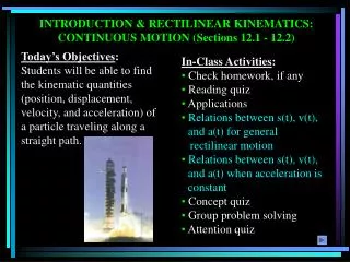
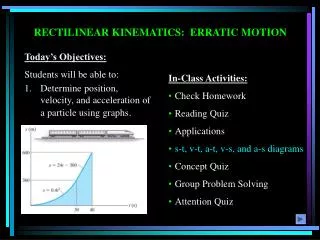
INTRODUCTION & RECTILINEAR KINEMATICS: CONTINUOUS MOTION • Today’s Objectives: • Students will be able to: • Find the kinematic quantities (position, displacement, velocity, and acceleration) of a particle traveling along a straight path.
Mechanics: The study of how bodies react to forces acting on them. Statics: The study of bodies in equilibrium. Dynamics: 1. Kinematics – concerned with the geometric aspects of motion 2. Kinetics - concerned with the forces causing the motion An Overview of Mechanics
Kinematics is the branch of classical mechanics that describes the motion of points, bodies (objects) and systems of bodies (groups of objects) without consideration of the causes of motion. The study of kinematics is often referred to as the geometry of motion. To describe motion, kinematics studies the trajectories of points, lines and other geometric objects and their differential properties such as velocity and acceleration. In mechanical engineering, robotics and biomechanics[8] to describe the motion of systems composed of joined parts (multi-link systems) such as an engine, a robotic arm or the skeleton of the human body.
The displacement of the particle is defined as its change in position. Vector form: r = r’ - r Scalar form: s = s’ - s RECTILINEAR KINEMATICS: CONTINIOUS MOTION (Section 12.2) A particle travels along a straight-line path defined by the coordinate axis s. The position of the particle at any instant, relative to the origin, O, is defined by the position vector r, or the scalar s. Scalar s can be positive or negative. Typical units for r and s are meters (m) or feet (ft). The totaldistancetraveled by the particle, sT, is a positive scalar that represents the total length of the path over which the particle travels.
The average velocity of a particle during a time interval t is vavg = r / t The instantaneous velocity is the time-derivative of position. v = dr / dt Speed is the magnitude of velocity: v = ds /dt It is how the position of a point changes with each instant of time. speed is also non-negative. VELOCITY Velocity is a measure of the rate of change in the position of a particle. It is a vector quantity (it has both magnitude and direction). The magnitude of the velocity is called speed, with units of m/s or ft/s. Average speed is the total distance traveled divided by elapsed time: (vsp)avg = sT / t
The instantaneous acceleration is the time derivative of velocity. Vector form: a= dv / dt Scalar form: a = dv / dt = d2s / dt2 Acceleration can be positive (speed increasing) or negative (speed decreasing). ACCELERATION Acceleration is the rate of change in the velocity of a particle. It is a vector quantity. Typical units are m/s2 or ft/s2. As the book indicates, the derivative equations for velocity and acceleration can be manipulated to get a ds = v dv
Position: Velocity: v t v s s t ò ò ò ò ò ò = = = dv a dt or v dv a ds ds v dt v o v s s o o o o o SUMMARY OF KINEMATIC RELATIONS: RECTILINEAR MOTION •Differentiate position to get velocity and acceleration. v = ds/dt ; a = dv/dt or a = v dv/ds •Integrate acceleration for velocity and position. • Note that so and vo represent the initial position and velocity of the particle at t = 0.
CONSTANT ACCELERATION The three kinematic equations can be integrated for the special case when accelerationis constant (a = ac) to obtain very useful equations. A common example of constant acceleration is gravity; i.e., a body freely falling toward earth. In this case, ac = g = 9.81 m/s2 = 32.2 ft/s2 downward. These equations are: v t ò ò = = + dv a dt v v a t yields c o c v o o s t ò ò = = + + (1/2) a ds v dt s s v t t yields o o c 2 s o o v s ò ò = = + v dv a ds v (v ) 2a (s - s ) yields 2 2 c o c o v s o o
Procedure for Analysis Coordinate System. • Establish a position coordinate s along the path and specify its fixed origin and positive direction. • Since motion is along a straight line, the vector quantities position, velocity, and acceleration can be represented as algebraic scalars. For analytical work the sense of s, v, and a is then defined by their algebraic signs. • The positive sense for each of these scalars can be indicated by an arrow shown alongside each kinematic equation as it is applied. Kinematic Equations. • If a relation is known between any two of the four variables a, v, s and t, then a third variable can be obtained by using one of the kinematic equations, a = dv/ dt, v = ds/ dt or a ds = v dv, since each equation relates all three variables. * • Whenever integration is performed, it is important that the position and velocity be known at a given instant in order to evaluate either the constant of integration if an indefinite integral is used, or the limits of integration if a definite integral is used. • Remember that Eqs. 12-4 through 12-6 have only limited use. These equations apply only when the acceleration is constant and the initial conditions are s = So and v = Vo when t = O.
EXAMPLE Given: A particle travels along a straight line to the right with a velocity of v = ( 4 t – 3 t2 ) m/s where t is in seconds. Also, s = 0 when t = 0. Find: The position and acceleration of the particle when t = 4 s. Plan: Establish the positive coordinate, s, in the direction the particle is traveling. Since the velocity is given as a function of time, take a derivative of it to calculate the acceleration. Conversely, integrate the velocity function to calculate the position.
EXAMPLE (continued) Solution: 1) Take a derivative of the velocity to determine the acceleration. a = dv / dt = d(4 t – 3 t2) / dt =4 – 6 t => a = – 20 m/s2 (or in the direction) when t = 4 s 2) Calculate the distance traveled in 4s by integrating the velocity using so = 0: v = ds / dt => ds = v dt => => s – so = 2 t2– t3 => s – 0 = 2(4)2– (4)3 => s = – 32 m ( or ) s t ò ò = ds (4 t – 3 t2) dt s o o
GROUP PROBLEM SOLVING Given: Ball A is released from rest at a height of 40 ft at the same time that ball B is thrown upward, 5 ft from the ground. The balls pass one another at a height of 20 ft. Find: The speed at which ball B was thrown upward. Plan: Both balls experience a constant downward acceleration of 32.2 ft/s2 due to gravity. Apply the formulas for constant acceleration, with ac = -32.2 ft/s2.
GROUP PROBLEM SOLVING (continued) Solution: 1) First consider ball A. With the origin defined at the ground, ball A is released from rest ((vA)o = 0) at a height of 40 ft ((sA )o = 40 ft). Calculate the time required for ball A to drop to 20 ft (sA = 20 ft) using a position equation. sA = (sA )o + (vA)o t + (1/2) ac t2 So, 20 ft = 40 ft + (0)(t) + (1/2)(-32.2)(t2) => t = 1.115 s
GROUP PROBLEM SOLVING (continued) Solution: 2) Now consider ball B. It is throw upward from a height of 5 ft ((sB)o = 5 ft). It must reach a height of 20 ft (sB = 20 ft) at the same time ball A reaches this height (t = 1.115 s). Apply the position equation again to ball B using t = 1.115s. sB = (sB)o + (vB)ot + (1/2) ac t2 So, 20 ft = 5 + (vB)o(1.115) + (1/2)(-32.2)(1.115)2 => (vB)o = 31.4 ft/s
End of the Lecture Example 12.1/2/3/4/5 textbook