Maximum likelihood decoding
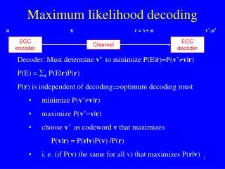
Maximum likelihood decoding. v. r = v+ n. u. v’,u’. ECC encoder. ECC decoder. Channel. Decoder: Must determine v’ to minimize P(E| r )=P( v ’ v | r ) P(E) = r P(E| r )P( r ) P( r ) is independent of decodingoptimum decoding must minimize P( v ’ v | r ) maximize P( v ’= v | r )

Maximum likelihood decoding
E N D
Presentation Transcript
Maximum likelihood decoding v r = v+ n u v’,u’ ECC encoder ECC decoder Channel • Decoder: Must determine v’ to minimize P(E|r)=P(v’v|r) • P(E) = r P(E|r)P(r) • P(r) is independent of decodingoptimum decoding must • minimize P(v’v|r) • maximize P(v’=v|r) • choose v’ as codeword v that maximizes • P(v|r) = P(r|v)P(v) /P(r) • i. e. (if P(v) the same for all v) that maximizes P(r|v)
ML decoding (cont.) • DMC: • P(r|v) = jP(rj|vj)…. • ML decoder: Choose v to maximize this expression • …or log P(r|v) = jlogP(rj|vj)…. • Is an ML decoder optimum? • Only if all v are equally probable as input vectors
ML decoding on BSC • BSC: • P(rj|vj) = 1-p if rj=vj, , p otherwise • log P(r|v) = jlogP(rj|vj) • Hamming distance: Let r and v differ in d(r,v) positions • jlogP(rj|vj) = d(r,v) log p + (n-d(r,v))log(1-p)= d(r,v) log (p/(1-p)) + nlog(1-p) • log (p/(1-p)) < 0 for p<0.5, so an ML decoder for a BSC must choose v to minimize d(r,v)
Channel capacity • Shannon (1948) • Every channel has a capacity C (determined by noise and available bandwidth) • Eb(R) is a positive function of R for R<C • There exists a block code of length n such that with ML decoding • P(E) < 2–nEb(R) • Similar for convolutional codes • In fact the average code performs like this. Nonconstructive proof • But ML decoding for long random codes is infeasible!
Performance measures • Tradeoff of main parameters: • Code rate • Error probability • Word error rate (WER, FER, BLER) • Bit error rate (BER) • at a given channel and channel quality • Decoding complexity • Performance is often displayed as a curve of an error rate as a function of channel quality
Error rate curves Log ER uncoded Coding threshold Shannon limit Coding gain SNR : Eb/N0 (dB) Eb=Es/R
Asymptotic coding gain Log ER Coding gain Asymptotic coding gain SNR : Eb/N0 (dB) uncoded
Asymptotic coding gain • High SNR, coded with soft-decision decoding: • Asymptotic coding gain: • ...or 10 log10 (Rdmin). For HD decoding: 10 log10 (Rdmin/2) • Thus SD gives 10 log10 2 = 3dB better ACG than HD
Performance close to the Shannon bound Log ER uncoded Shannon limit SNR : Eb/N0 (dB) Classical code Turbo code or LDPC code
Coded modulation • Encoding + modulation: • Need a distance preserving modulation mapping, preserving distance between different codewords • Thus we can view codes also in the modulation domain • Combined coding and modulation: Design codes specifically to increase distance • Exploit that in a large signal constellation some points are further apart
Coded modulation • Some schemes work on a signal constellation by: • Encode some input bits by an ECC. Let the output bits determine a subconstellation • Let the remaining input bits determine a point in the subconstellation • TCM – coded modulation based on a convolutional ECC • BCM – coded modulation based on block ECC • Also: coded modulation with turbo codes and LDPC codes
Trellises of linear block codes (CH 9) Receiver Sender 0 0 0 01 1 10 1 1 1 0 E E E O O • A representation that facilitates soft-decision decoding • Recall: • A linear block code is the row space of a generator matrix • Example: E
Trellises • A trellis is a directed graph: • A set of depths or time instances, ordered (usually) from 0 to n • At each time instant, a set of nodes, vertices, representing the (code) state at that time instant. Usually (in an ordinary block code) one initial state s0 at time instant 0 and one final state sf at time n • Edges can go from a state at time i to a state at time i+1 • Each edge is labeled by one (or more) symbol(s) from the code alphabet (usually binary) • A sequence of edge labels obtained by traversing the trellis from s0 to sf is a codeword
Linear trellises si+1 Oi si • Necessary (but not sufficient) conditions for a trellis (or corresponding code) to be linear: • Oi= fi(si, Ii) • Output block Oi • Input block Ii • State si at time instant i • Depends on time instant • si+1= gi(si, Ii)
More properties of linear trellises • In the trellis of a linear code, the set of states i at time i is called the state space • A trellis is time invariant iff • a finite period initial delay • An output function f and a state transition function g • a ”template”state space • such that • i for i < , and i = for i • fi=f and gi=g for all i
Bit-level trellises of linear block codes • [n,k] code C • Bit-level trellis: n+1 time instants and n trellis sections • One initial state s0 at time 0, one final state sf at time n • For each time i >0, there is a fixed number Incoming(i) of incoming branches. For all i, Incoming(i) is 1 or 2. Two branches going to the same state have different labels. • For each time i <n, there is a fixed number Outgoing(i) of outgoing branches. For all i, outgoing(i) is 1 or 2. Two branches coming from the same state have different labels. • Each codeword corresponds to a distinct path from s0 to sf
Bit-level trellises of linear block codes • The number |i| is (sometimes) called the state space complexity at time instant i. For a linear code, we will show that |i| for all i , |i| is a power of 2 • Thus we can define the state space dimension • i = log2|i| • The sequence ( 0=0, 1 ,..., i,..., n=0) is called the state space dimension profile, and determines the complexity of a maximum likelihood (soft-decision) decoder for the code.

