Maximum Likelihood Estimation

1. Maximum Likelihood Estimation Psych 818 - DeShon

2. MLE vs. OLS • Ordinary Least Squares Estimation • Typically yields a closed form solution that can be directly computed • Closed form solutions often require very strong assumptions • Maximum Likelihood Estimation • Default Method for most estimation problems • Generally equal to OLS when OLS assumptions are met • Method yields desirable “asymptotic” estimation properties • Foundation for Bayesian inference • Requires numerical methods :(

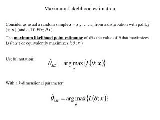
3. MLE logic • MLE reverses the probability inference • Recall: p(X|) •  represents the parameters of a model (i.e., pdf) • What’s the probability of observing a score of 73 from a N(70,10) distribution • In MLE, you know the data (Xi) • Primary question: Which of a potentially infinite number of distributions is most likely responsible for generating the data? • p(|X)?

4. Likelihood • Likelihood may be thought of as an unbounded or unnormalized probability measure • PDF is a function of the data given the parameters on the data scale • Likelihood is a function of the parameters given the data on the parameter scale

5. Likelihood • Likelihood function • Likelihood is the joint (product) probability of the observed data given the parameters of the pdf • Assume you have X1,…,Xn independent samples from a given pdf, f

6. Likelihood • Log-Likelihood function • Working with products is a pain • maxima are unaffected by monotone transformations, so can take the logarithm of the likelihood and turn it into a sum

7. Maximum Likelihood • Find the value(s) of  that maximize the likelihood function • Can sometimes be found analytically • Maximization (or minimization) is the focus of calculus and derivatives of functions • Often requires iterative numeric methods

8. Likelihood • Normal Distribution example • pdf: • Likelihood • Log-Likelihood • Note: C is a constant that vanishes once derivatives are taken

9. Likelihood • Can compute the maximum of this log-likelihood function directly • More relevant and fun to estimate it numerically!

10. Normal Distribution example • Assume you obtain 100 samples from a normal distribution • rv.norm <- rnorm(100, mean=5, sd=2) • This is the true data generating model! • Now, assume you don’t know the mean of this distribution and we have to estimate it… • Let’s compute the log-likelihood of the observations for N(4,2)

11. Normal Distribution example • sum(dnorm(rv.norm, mean=4, sd=2, log=T)) • dnorm gives the probability of an observation for a given distribution • Summing it across observations gives the log-likelihood • = -221.0698 • This is the log-likelihood of the data for the given pdf parameters • Okay, this is the log-likelihood for one possible distribution….we need to examine it for all possible distributions and select the one that yields the largest value

12. Normal Distribution example • Make a sequence of possible means • m<-seq(from = 1, to = 10, by = 0.1) • Now, compute the log-likelihood for each of the possible means • This is a simple “grid search” algorithm • log.l<-sapply(m, function (x) sum(dnorm(rv.norm, mean=x, sd=2, log=T)) )

13. Normal Distribution example mean log.l 1 1.0 -417.3891 2 1.1 -407.2201 3 1.2 -397.3012 4 1.3 -387.6322 5 1.4 -378.2132 6 1.5 -369.0442 7 1.6 -360.1253 8 1.7 -351.4563 9 1.8 -343.0373 10 1.9 -334.8683 11 2.0 -326.9494 12 2.1 -319.2804 13 2.2 -311.8614 14 2.3 -304.6924 15 2.4 -297.7734 16 2.5 -291.1045 17 2.6 -284.6855 18 2.7 -278.5165 19 2.8 -272.5975 20 2.9 -266.9286 21 3.0 -261.5096 22 3.1 -256.3406 23 3.2 -251.4216 24 3.3 -246.7527 25 3.4 -242.3337 26 3.5 -238.1647 27 3.6 -234.2457 28 3.7 -230.5768 29 3.8 -227.1578 30 3.9 -223.9888 31 4.0 -221.0698 32 4.1 -218.4008 33 4.2 -215.9819 34 4.3 -213.8129 35 4.4 -211.8939 36 4.5 -210.2249 37 4.6 -208.8060 38 4.7 -207.6370 39 4.8 -206.7180 40 4.9 -206.0490 41 5.0 -205.6301 42 5.1 -205.4611 43 5.2 -205.5421 44 5.3 -205.8731 45 5.4 -206.4542 46 5.5 -207.2852 47 5.6 -208.3662 48 5.7 -209.6972 49 5.8 -211.2782 50 5.9 -213.1093 51 6.0 -215.1903 52 6.1 -217.5213 53 6.2 -220.1023 54 6.3 -222.9334 55 6.4 -226.0144 56 6.5 -229.3454 57 6.6 -232.9264 58 6.7 -236.7575 59 6.8 -240.8385 60 6.9 -245.1695 61 7.0 -249.7505 62 7.1 -254.5816 63 7.2 -259.6626 64 7.3 -264.9936 65 7.4 -270.5746 66 7.5 -276.4056 67 7.6 -282.4867 68 7.7 -288.8177 69 7.8 -295.3987 70 7.9 -302.2297 71 8.0 -309.3108 72 8.1 -316.6418 73 8.2 -324.2228 74 8.3 -332.0538 75 8.4 -340.1349 76 8.5 -348.4659 77 8.6 -357.0469 78 8.7 -365.8779 79 8.8 -374.9590 80 8.9 -384.2900 81 9.0 -393.8710 82 9.1 -403.7020 83 9.2 -413.7830 84 9.3 -424.1141 85 9.4 -434.6951 86 9.5 -445.5261 87 9.6 -456.6071 88 9.7 -467.9382 89 9.8 -479.5192 90 9.9 -491.3502 91 10.0 -503.4312 Why are these numbers negative?

14. Normal Distribution example • dnorm gives us the probability of an observation from the given distribution • The log of a value between 0-1 is negative • Log(.05)=-2.99 • What’s the MLE? • m[which(log.l==max(log.l))] • = 5.1

15. Normal Distribution example • What about estimating both the mean and the SD simultaneously? • Use grid search approach again… • Compute the log-likelihood at each combination of mean and SD SD Mean log.l 1 1.0 1.0 -1061.6201 2 1.0 1.1 -1022.2843 3 1.0 1.2 -983.9486 4 1.0 1.3 -946.6129 5 1.0 1.4 -910.2771 6 1.0 1.5 -874.9414 7 1.0 1.6 -840.6056 8 1.0 1.7 -807.2699 9 1.0 1.8 -774.9341 10 1.0 1.9 -743.5984 11 1.0 2.0 -713.2627 12 1.0 2.1 -683.9269 13 1.0 2.2 -655.5912 14 1.0 2.3 -628.2554 15 1.0 2.4 -601.9197 16 1.0 2.5 -576.5839 17 1.0 2.6 -552.2482 18 1.0 2.7 -528.9125 19 1.0 2.8 -506.5767 20 1.0 2.9 -485.2410 853 1.9 4.3 -211.3830 854 1.9 4.4 -209.6280 855 1.9 4.5 -208.1499 856 1.9 4.6 -206.9489 857 1.9 4.7 -206.0249 858 1.9 4.8 -205.3779 859 1.9 4.9 -205.0078 860 1.9 5.0 -204.9148 861 1.9 5.1 -205.0988 862 1.9 5.2 -205.5599 863 1.9 5.3 -206.2979 864 1.9 5.4 -207.3129 865 1.9 5.5 -208.6049 866 1.9 5.6 -210.1740 867 1.9 5.7 -212.0200 868 1.9 5.8 -214.1431 869 1.9 5.9 -216.5432 870 1.9 6.0 -219.2203 871 1.9 6.1 -222.1743 872 1.9 6.2 -225.4054 873 1.9 6.3 -228.9135 6134 7.7 4.6 -299.1132 6135 7.7 4.7 -299.0569 6136 7.7 4.8 -299.0175 6137 7.7 4.9 -298.9950 6138 7.7 5.0 -298.9893 6139 7.7 5.1 -299.0006 6140 7.7 5.2 -299.0286 6141 7.7 5.3 -299.0736 6142 7.7 5.4 -299.1354 6143 7.7 5.5 -299.2140 6144 7.7 5.6 -299.3096 6145 7.7 5.7 -299.4220 6146 7.7 5.8 -299.5512 6147 7.7 5.9 -299.6974 6148 7.7 6.0 -299.8604 6149 7.7 6.1 -300.0402 6150 7.7 6.2 -300.2370 6151 7.7 6.3 -300.4506

16. Normal Distribution example • Get max(log.l) • m[which(log.l==max(log.l), arr.ind=T)] • = 5.0, 1.9 • Note: this could be done the same way for a simple linear regression (2 parameters)

17. Algorithms • Grid search works for these simple problems with few estimated parameters • Much more advanced search algorithms are needed for more complex problems • More advanced algs take advantage of the slope or gradient of the likelihood surface to make good guesses about the direction of search in parameter space • We’ll use the “mlm” routine in R

18. Algorithms • Grid Search: • Vary each parameter in turn, compute the log-likelihood, then find parameter combination yielding lowest log-likelihood • Gradient Search: • Vary all parameters simultaneously, adjusting relative magnitudes of the variations so that the direction of propagation in parameter space is along the direction of steepest ascent of log-likelihood • Expansion Methods: • Find an approximate analytical function that describes the log-likelihood hypersurface and use this function to locate the minimum. Number of computed points is less, but computations are considerably more complicated. • Marquardt Method: Gradient-Expansion combination

19. R – mlm routine • First we need to define a function to maximize • Wait! Most general routines focus on minimization • e.g., root finding for solving equations • So, usually minimize –log-likelihood • norm.func<-function(x,y) {   sum(sapply(rv.norm, function(z) -1*dnorm(z, mean=x, sd=y, log=T))) }

20. R – mlm routine • norm.mle <- mle(norm.func, start=list(x=4,y=2), method="L-BFGS-B", lower=c(0, 0)) • Many interesting points • Starting values • Global vs. local maxima or minima • Bounds • SD can’t be negative

21. R – mlm routine • Output - summary(norm.mle) • Standard errors come from the inverse of the hessian matrix • Convergence!! • -2(log-likelihood) = deviance • Functions like the R2 in regression Coeficients: Estimate Std. Error x 4.844249 0.1817031 y 1.817031 0.1284834 -2 log L: 403.2285 > norm.mle@details$convergence [1] 0

22. Maximum Likelihood Regression • A standard regression: • May be broken down into two components

23. Maximum Likelihood Regression • First define our x's and y'sx<- 1:100 y<- 4 + 3*x+rnorm(100, mean=5, sd=20) • Define -log likelihood function reg.func <- function(b0,b1,sigma) {   if(sigma<=0) return(NA) # no sd of 0 or less!   yhat<-b0*x+b1 #the estimated function   -sum(dnorm(y, mean=yhat, sd=sigma,log=T)) #the -log likelihood function }

24. Maximum Likelihood Regression • Call MLE to minimize the –log-likelihood lm.mle<-mle(reg.func, start=list(b0=2, b1=2, sigma=35)) • Get results - summary(lm.mle) Coefficients: Estimate Std. Error b0 3.071449 0.0716271 b1 8.959386 4.1663956 sigma 20.675930 1.4621709 -2 log L: 889.567

25. Maximum Likelihood Regression • Compare to OLS results • lm(y~x) Coefficients: Estimate Std. Error t value Pr(>|t|) (Intercept) 8.95635 4.20838 2.128 0.0358 * x 3.07149 0.07235 42.454 <2e-16 *** --- Signif. codes: 0 ‘***’ 0.001 ‘**’ 0.01 ‘*’ 0.05 ‘.’ 0.1 ‘ ’ 1 Residual standard error: 20.88 on 98 degrees of freedom Multiple R-Squared: 0.9484,

26. Standard Errors of Estimates • Behavior of the likelihood function near the maximum is important • If it is flat then observations have little to say about the parameters • changes in the parameters will not cause large changes in the probability • if the likelihood has a pronounced peak near to the maximum then small changes in parameters would cause large changes in probability • In this cases we say that observation has more information about parameters • Expressed as the second derivative (or curvature) of the log-likelihood function • If more than 1 parameter, then 2nd partial deriviatives

27. Standard Errors of Estimates • Rate of change is the second derivative of a function (e.g., velocity and acceleration) • Hessian Matrix is the matrix of 2nd partial derivatives of the -log-likelihood function • The entries in the Hessian are called the observed information for an estimate

28. Standard Errors • Information is used to obtained the expected variance (or standard error) or the estimated parameters • When sample size becomes large then maximum likelihood estimator becomes approximately normally distributed with variance close to • More precisely…

29. Likelihood Ratio Test • Let LF be the maximum of the likelihood function for an unrestricted model • Let LR be the maximum of the likelihood function of a restricted model nested in the full model • LF must be greater than or equal to LR • Removing a variable or adding a constraint can only hurt model fit. Same logic as R2 • Question: Does adding the constraint or removing the variable (constraint of zero) significantly impact model fit? • Model fit will decrease but does it decrease more than would be expected by chance?

30. Likelihood Ratio Test • Likelihood Ratio • R = -2ln(LR / LF) • R = 2(log(LF) – log(LR)) • R is distributed as chi-square distribution with m degrees of freedom • m is the difference in the number of estimated parameters between the two models. • The expected value of R is m, so if you get an R that is bigger than the difference in parameters then the constraint hurts model fit. • More formally…. You should reference the chi-square table with m degrees of freedom to find the probability of getting R by chance alone, assuming that the null hypothesis is true.

31. Likelihood Ratio Example • Go back to our simple regression example • Does the variable (X) significantly improve our predictive ability or model fit? • Alternatively, does removing X or constraining it’s parameter estimate to zero significantly decrease prediction or model fit? • Full Model: -2log-L = 889.567 • Reduced Model: -2log-L =1186.05 • Chi-square critical value = 3.84

32. Fit Indices • Akaike’s information criterion (AIC) • Pronounced “Ah-kah-ee-key” • K is the number of estimated parameters in our model. • Penalizes the log-likelihood for using many parameters to increase fit • Choose the model with the smallest AIC value

33. Fit Indices • Bayesian Information Criterion (BIC) • AKA- SIC for Schwarz Information Criterion • Choose the model with the smallest BIC • the likelihood is the probability of obtaining the data you did under the given model. It makes sense to choose a model that makes this probability as large as possible. But putting the minus sign in front switches the maximization to minimization

34. Multiple Regression • -Log-Likelihood function for multiple regression #Note, theta is a vector of parameters, with std.dev being the first one#theta[-1] is all values of theta, except the first#and here we're using matrix multiplication ols.lf3 <- function(theta, y, X) {   if (theta[1] <= 0) return(NA)   -sum(dnorm(y, mean = X %*% theta[-1], sd = sqrt(theta[1]), log = TRUE))}