Maximum-Likelihood estimation

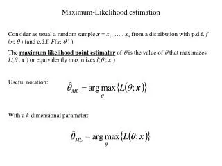
1. Maximum-Likelihood estimation Consider as usual a random sample x = x1, … , xnfrom a distribution with p.d.f. f (x;  ) (and c.d.f. F(x;  ) ) The maximum likelihood point estimatorof  is the value of  that maximizes L( ; x) or equivalently maximizes l( ; x) Useful notation: With a k-dimensional parameter:

2. Complete sample case: If all sample values are explicitly known, then Censored data case: If some ( say nc)of the sample values are censored , e.g. xi< k1 or xi> k2 , then where

3. When the sample comes from a continuous distribution the censored data case can be written In the case the distribution is discrete the use of F is also possible: If k1 and k2 are values that can be attained by the random variables then we may write where

4. Example:

5. Example: Solution must be numerically found

6. For the exponential family of distributions: Use the canonical form (natural parameterization): Let Then the maximum likelihood estimators (MLEs) of 1, … , k are found by solving the system of equations

7. Example:

9. Computational aspects • When the MLEs can be found by evaluating • numerical routines for solving the generic equation g( ) = 0 can be used. • Newton-Raphson method • Fisher’s method of scoring (makes use of the fact that under regularity conditions: • ) • This is the multidimensional analogue of Lemma 2.1 ( see page 17)

10. When the MLEs cannot be found the above way other numerical routines must be used: • Simplex method • EM-algorithm • For description of the numerical routines see textbook. • Maximum Likelihood estimation comes into natural use not for handling the standard case, i.e. a complete random sample from a distribution within the exponential family , but for finding estimators in more non-standard and complex situations.

11. Example:

12. Properties of MLEs Invariance: Consistency: Under some weak regularity conditionsall MLEs are consistent Efficiency: Under the usual regularity conditions: (Asymptotically efficient and normally distributed)

13. Sufficiency: Example:

15. Invariance property 

18. i.e. the two MLEs are asymptotically uncorrelated (and by the normal distribution independent)

19. Modifications and extensions Ancillarity and conditional sufficiency:

20. Profile likelihood: This concept has its main use in cases where  1 contains the parameters of “interest” and  2 contains nuisance parameters. The same ML point estimator for  1 is obtained by maximizing the profile likelihood as by maximizing the full likelihood function

21. Marginal and conditional likelihood: Again, these concepts have their main use in cases where  1 contains the parameters of “interest” and  2 contains nuisance parameters.

22. Penalized likelihood: MLEs can be derived subjected to some criteria od smoothness. In particulare this is applicable when the parameter is no longer a single value (one- or multidimensional), but a function such as an unknown density function or a regression curve. The penalized log-likelihood function is written

23. Method of moments estimation (MM )

24. The method of moments point estimator of  = ( 1, … ,  k ) is obtained by solving for  1, … ,  k the systems of equations

25. Example:

27. Method of Least Squares (LS) First principles: Assume a sample xwhere the random variable Xi can be written The least-squares estimator of  is the value of  that minimizes i.e.

28. A more general approach: Assume the sample can be written (x, z ) where xirepresents the random variable of interest (endogenous variable) and zi represent either an auxiliary random variable (exogenous) or a given constant for sample point i The least squares estimator of  is then

29. Special cases: The ordinary linear regression model: The heteroscedastic regression model:

30. The first-order auto-regressive model: The conditional least-squares estimator of  (given ) is