Comparing Methods for Identifying Transcription Factor Target Genes
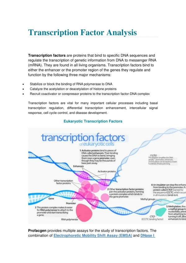
280 likes | 402 Vues
This presentation provides an overview of various methods for identifying transcription factor (TF) target genes. We explore computational techniques like Position Weight Matrix (PWM) genome scanning and TRAP for binding affinity predictions, as well as experimental approaches such as microarrays and ChIP-seq. Each method's advantages and limitations are discussed, including the necessity for biological validation and the complexities involved in analyzing TF binding sites. Understanding these methods is crucial for accurately determining gene regulation mechanisms influenced by transcription factors.

Comparing Methods for Identifying Transcription Factor Target Genes
E N D
Presentation Transcript
Comparing Methods for Identifying Transcription Factor Target Genes • Alena van Bömmel(R 3.3.73) • Matthew Huska (R 3.3.18) • Max Planck Institute for Molecular Genetics
Transcriptional Regulation TF notbound = no gene expression TF bound = gene expression
Transcriptional Regulation TF notbound = no gene expression TF bound = gene expression Problem: There are many genes and many TF's, how do we identify the targets of a TF?
Methods for Identifying TF Target Genes PWM Genome Scan Microarray ChIP-seq
PWM Genome Scan • Purely computational method • Input: • position weight matrix for your TF • genomic region(s) of interest • Pros: • No need to do wet lab experiments • Cons: • Many false positives, not able to take biological conditions into account Score threshold
PWM genome scan • Download the PWMs of your TF of interest from the database (they might include >1 motif) • Define the sequences to analyze (promoter sequences) • Run the PWM genome scan (hit-based method or affinity prediction method) • Rank the genomic sequences by the affinity signal • Suggested Reading: • Roider et al.: Predicting transcription factor affinities to DNA from a biophysical model. Bioinformatics (2007). • Thomas-Chollier et al.Transcription factor binding predictions using TRAP for the analysis of ChIP-seq data and regulatory SNPs. Nature Protocols (2011).
TRAP • Convert the PSSM(position specific scoring matrix) to PSEM (position specific energy matrix) • Scan the sequences of interest with TRAP • Results in 1 score per sequence=binding affinity • Doesn’t separate the exact TF binding sites (easier for ranking) • Sequences must have the same length! ANNOTATE=/project/gbrowse/Pipeline/ANNOTATE_v3.02/Release TRAP trap.molgen.mpg.de/cgi-bin/home.cgi
Matrix-scan • Use directly the PSSM • Finds all TFBS which exceed a predefined threshold (e.g. p-value) • More complicated to create ranked lists of genomic sequences (more hits in the sequence) • Exact location of the binding site reported matrix-scan http://rsat.ulb.ac.be/
Finding the target genes • target genes will be the top-ranked genes (promoters) • which are the top-ranked genes? (top-100,500,1000...?) • There’s no exact definition of promoters, usually 2000bp upstream, 500bp downstream of the TSS
Microarrays → R/Bioconductor (details later)
Folie 12 Microarrays (2) • Pros: • There is a lot of microarray data already available (might not have to generate the data yourself) • Inexpensive and not very difficult to perform • Computational workflow is well established • Cons: • Can not distinguish between indirect regulation and direct regulation
ChIP-seq Map reads to the genome Call peaks to determine most likely TF binding locations
Folie 14 ChIP-seq (2) • Pros: • Direct measure of genome-wide protein-DNA interaction(*) • Cons: • Don't know whether binding causes changes in gene expression • More complicated experimentally and in terms of computational analysis • Most expensive • Need an antibody against your protein of interest • Biases are not as well understood as with microarrays
ChIP-seq analysis • Download the reads from given source (experiments and controls) • Quality control of the reads and statistics (fastqc) • Mapping the reads to the reference genome (bwa/Bowtie) • Peak calling (MACS) • Visualization of the peaks in a genome browser (genome browser, IGV) • Finding the closest genes to the peaks(Bioconductor/ChIPpeakAnno) Visualised peaks in a genome browser • Suggested Reading: • Bailey et alPracticalGuidelines for the Comprehensive Analysis of ChIP-seq Data.PLoSComputBiol(2013). • Thomas-Chollier et al. A complete workflow for the analysis of full-size ChIP-seq (and similar) data sets using peak-motifs.Nature Protocols (2012).
Sequencing data • raw data=reads usually very large file (few GB) • formatfastq (ENCODE) or SRA (Sequence Read Archive of NCBI) Analysis • Quality control with fastqc • Filteringof reads with adapter sequences • Mapping of the reads to the reference genome (bwa or Bowtie) Example of fastq data file
Quality control with fastqc • per base quality • sequence quality (avg. > 20) • sequence length • sequence duplication level (duplication by PCR) • overrepresented sequences/kmers (adapter sequences) • produces a html report • manual(read it!) • software at the MPI Example of per base seq quality scores FASTQC=/scratch/ngsvin/bin/chip-seq/fastqc/FastQC/fastqc
Mapping with bwa • mapping the sequencing reads to a reference genome • manual(read it!) • map the experiments and the controls • reference genome in fasta format (hg19) • create an index of the reference file for faster mapping (only if not available) • align the reads (specify parameters e.g. for # of mismatches, read trimming, threads used...) • generate alignments in the SAM format (different commands for single-end and pair-end reads!) • software and data at the MPI: BWA = /scratch/ngsvin/bin/executables/bwa hg19: /scratch/ngsvin/MappingIndices/hg19.fa bwaindex: /scratch/ngsvin/MappingIndices/BWA/hg19
File manipulation with samtools • utilities that manipulate SAM/BAM files • manual (read it!) • merge the replicates in one file (still separate experiment and control) • convert the SAM file into BAM file (binary version of SAM, smaller) • sort and index the BAM file • now the sequencing files are ready for further analysis • software at the MPI: SAMTOOLS = /scratch/ngsvin/bin/executables/samtools
Peak finding with MACS • find the peaks, i.e. the regions with a high density of reads, where the studied TF was bound • manual(read it!) • call the peaks using the experiment (treatment) data vs. control • set the parameters e.g. fragment length, treatment of duplication reads • analyse the MACS results (BED file with peaks/summits) • software at the MPI: MACS = /scratch/ngsvin/bin/executables/macs
Finding the target genes • find the genes which are in the closest distance to the (significant) peaks • how to define the closest distance? (+- X kb) • use ChIPpeakAnno in Bioconductor or bedtools
Methods for Identifying TF Target Genes PWM Genome Scan Microarray ChIP-seq Thresholds
Bioinformatics • Read mapping (Bowtie/bwa) • Peak Calling (MACS/Bioconductor) • Peak-Target Analysis (Bioconductor) • Microarray data analysis (Bioconductor) • Differential Genes (R) • GSEA • PWM Genome Scan (TRAP/MatScan) • Statistics (R) • Data Integration (R/Python/Perl) • Statistical Analysis (R)
Bioinformatics tools READ THE MANUALS! • Bowtiebowtie-bio.sourceforge.net/manual.shtml • bwabio-bwa.sourceforge.net/bwa.shtml • MACS github.com/taoliu/MACS/blob/macs_v1/README.rst • TRAPtrap.molgen.mpg.de/cgi-bin/home.cgi • matrix-scan http://rsat.ulb.ac.be/ • Bioconductorwww.bioconductor.org/(more info in R course) Databases • GEOwww.ncbi.nlm.nih.gov/geo/ • ENCODE genome.ucsc.edu/ENCODE/ • SRAwww.ncbi.nlm.nih.gov/sra • JASPAR http://jaspar.genereg.net/
Schedule • 03.03. Introduction lecture, R course • 04.03. R & Bioconductor homework submission • 11.03. Presentation of the detailed plan of each group (which TF, cell line, tools, data, data integration, team work ) 10:30am, 11:30am • every Tuesday 10:30am, 11:30am progress meetings • 17.04. Final report deadline • 24.04. (tentative) Presentations • 28.04. Final meeting, discussion of final reports
GR Group • Expression and ChIP-seqdata: Luca F, Maranville JC, et al., PLoS ONE, 2013 • PWM database: jaspar.genereg.net
c-Myc Group • Expression data: Cappellen, Schlange, Bauer et al., EMBO reports, 2007 • Musgrove et al., PLoS One, 2008 • ChIP-seq data: ENCODE Project • PWM database: jaspar.genereg.net
Additional analysis • Binding motifs • are the overrepresented motifs in the ChIP-peak regions different? • do we find any co-factors? • Recommended tool: • RSAT rsat.ulb.ac.be binding motifs binding motifs binding motifs