Inserting Data
Learn how to enter QB data, create formulas for stats like INT/TD, apply conditional formatting for player performance, and freeze panes in Excel for a complete football analysis.

Inserting Data
E N D
Presentation Transcript
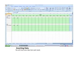
Inserting Data You will insert your data here each week.
Creating a formula Click the fx button to insert a formula. The above pop-up should appear. Select “OK” to enter a SUM.
Creating a formula When this pop-up appears, do NOT click anything. Click on the “QB Data” tab to return to your data entry screen. Once there, scroll over to Interceptions.
Creating a formula Once on the QB Data screen, highlight the column of Interceptions for the respective week for your first QB. (The reason we have more than one row is because you might switch your QB out for someone else later.
Creating a formula We’re halfway done with the formula. Since we’re doing INT/TD, put a “/” in the formula bar at the top of the screen following the equation you’ve already entered.
Creating a formula Once you’ve put in your slash, click the fx button again and perform the same procedure you did before (for TD’s this time).
Note: For Wk1, your “INT/TD”formula should look like: =SUM('QB Data'!AJ4:AJ9)/SUM('QB Data'!S4:S9) Your Yrds/Sack formula should look like: =SUM('QB Data'!B4:B9)/SUM('QB Data'!BA4:BA9) Conditional Formatting Once your formula is entered, you can make the cell turn red or green based on the player’s performance. Click on Conditional Formatting at the top of the page. If no rule is present, you will click ‘New Rule’. If you just want to change an existing rule, click ‘Manage Rules’.
Conditional Formatting Since ideally we want INT/TD to be a low #, we want to turn the cell GREEN if it is LESS than our standard and RED if it is GREATER than our standard.
Conditional Formatting Click ‘New Rule’, ‘Format only cells that contain’, and change your middle drop-down selection to ‘less than’. Enter your standard for INT/TD. As you can see, I have selected 1.5 INT/TD as the make-or-break for my QB’s.
3) Select the ‘Custom’ tab and set your Font color to 0-97-0. 2) Select ‘More Colors’ from the Color drop-down menu on the Font screen. 1) Click ‘Format’ Conditional Formatting Now let’s apply the font color.
3) Select the ‘Custom’ tab and set your Fill color to 198-239-206. 2) Select ‘More Colors’ from the Color drop-down menu on the Fill screen. 1) Click ‘Format’ Conditional Formatting Now let’s apply the fill color.
Conditional Formatting Perform the same steps for your RED condition, except this time, your condition will be if INT/TD is GREATER than 1.5. Your Font color should be 156-0-6 and your Fill 255-199-206.
This time under ‘Cells that contain’, select “Errors”. Since we want it RED, set your Fill to 255-199-206 and your Font to 156-0-6. Conditional Formatting Now’s the weird scenario. It is possible to have 0 TD’s, and you get an error because you are dividing by 0 (a big no-no). 0 TD’s is a bad statistic, so to fix this, we’ll make this situation turn RED.
Move rules up and down Stop if True Conditional Formatting Now, select ‘Manage Rules’ under Conditional Formatting. Order your Rules as I have done and select ‘Stop If True’ next to your Green condition at the top of the list.
Conditional Formatting Now perform the same above steps to set your QB’s Yrds/Sack conditions. Once you’re done, your list of rules should look like mine above. Note that my make-or-break value is 125 Yrds/Sack. Once you’ve done this, complete the same values for QB2.
I scrolled too far and the stat categories have disappeared. Freezing Panes Once you have all of your equations done, let’s flip to the last tab called TOTALS. It’d be nice to see the stat categories when I scroll all the way over to Wk17.
Freeze first column Freezing Panes To Fix this problem, select ‘Freeze Panes’ under the ‘View’ tab at the top of the page. Once selected, simply ‘Freeze the First Column’.