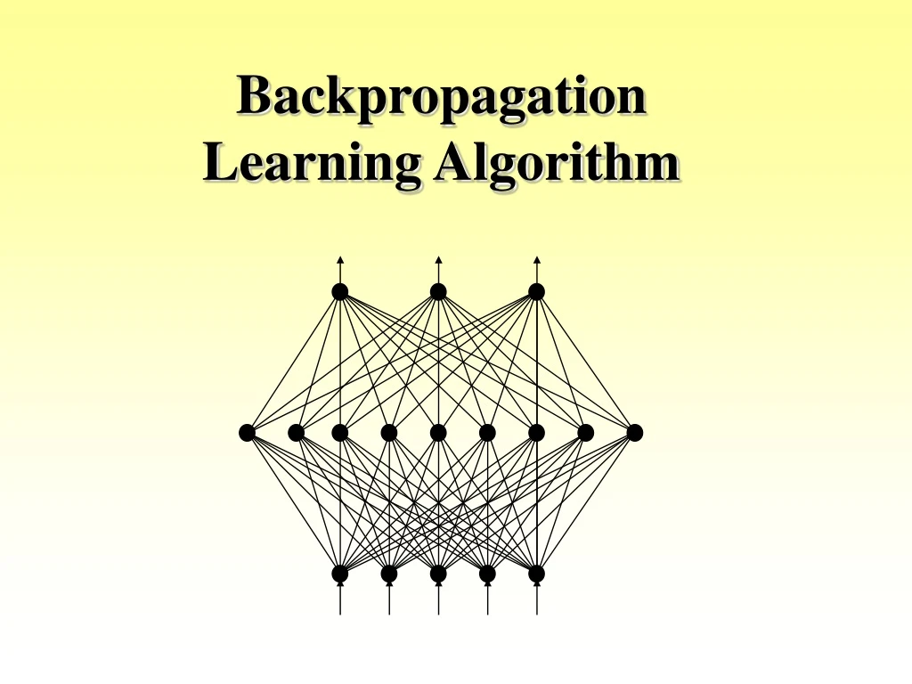

Backpropagation Learning Algorithm for Multi-Layer Perception
E N D
Presentation Transcript
x1 xn The backpropagation algorithm was used to train the multi layer perception MLP MLP used to describe any general Feedforward (no recurrent connections) Neural Network FNN However, we will concentrate on nets with units arranged in layers
Architecture of BP Nets • Multi-layer, feed-forward networks have the following characteristics: -They must have at least one hidden layer • Hidden units must be non-linear units (usually with sigmoid activation functions) • Fully connected between units in two consecutive layers, but no connection between units within one layer. • For a net with only one hidden layer, each hidden unit receives input from all input units and sends output to all output units • Number of output units need not equal number of input units • Number of hidden units per layer can be more or less than input or output units
Other Feedforward Networks • Madaline • Multiple adalines (of a sort) as hidden nodes • Adaptive multi-layer networks • Dynamically change the network size (# of hidden nodes) • Networks of radial basis function(RBF) • e.g., Gaussian function • Perform better than sigmoid function (e.g., interpolation in function approximation
Introduction to Backpropagation • In 1969 a method for learning in multi-layer network, Backpropagation (or generalized delta rule) , was invented by Bryson and Ho. • It is best-known example of a training algorithm. Uses training data to adjust weights and thresholds of neurons so as to minimize the networks errors of prediction. • Slower than gradient descent . • Easiest algorithm to understand • Backpropagation works by applying the gradient descent rule to a feedforward network.
How many hidden layers and hidden units per layer? • Theoretically, one hidden layer (possibly with many hidden units) is sufficient for any L2 functions • There is no theoretical results on minimum necessary # of hidden units (either problem dependent or independent) • Practical rule : • n = # of input units; p = # of hidden units • For binary/bipolar data: p = 2n • For real data: p >> 2n • Multiple hidden layers with fewer units may be trained faster for similar quality in some applications
Training a BackPropagation Net • Feedforward training of input patterns • each input node receives a signal, which is broadcast to all of the hidden units • each hidden unit computes its activation which is broadcast to all output nodes • Back propagation of errors • each output node compares its activation with the desired output • based on these differences, the error is propagated back to all previous nodes Delta Rule • Adjustment of weights • weights of all links computed simultaneously based on the errors that were propagated back
Generalized delta rule • Delta rule only works for the output layer. • Backpropagation, or the generalized delta rule, is a way of creating desired values for hidden layers
Description of Training BP Net: Feedforward Stage 1. Initialize weights with small, random values 2. While stopping condition is not true • for each training pair (input/output): • each input unit broadcasts its value to all hidden units • each hidden unit sums its input signals & applies activation function to compute its output signal • each hidden unit sends its signal to the output units • each output unit sums its input signals & applies its activation function to compute its output signal
Training BP Net:Backpropagation stage 3. Each output computes its error term, its own weight correction term and its bias(threshold) correction term & sends it to layer below 4. Each hidden unit sums its delta inputs from above & multiplies by the derivative of its activation function; it also computes its own weight correction term and its bias correction term
Training a Back Prop Net:Adjusting the Weights • Each output unit updates its weights and bias 6. Each hidden unit updates its weights and bias • Each training cycle is called an epoch. The weights are updated in each cycle • It is not analytically possible to determine where the global minimum is. Eventually the algorithm stops in a low point, which may just be a local minimum.
How long should you train? • Goal: balance between correct responses for training patterns & correct responses for new patterns (memorization v. generalization) • In general, network is trained until it reaches an acceptable error rate (e.g. 95%) • If train too long, you run the risk of overfitting
Graphical description of of training multi-layer neural network using BP algorithm To apply the BP algorithm to the following FNN
To teach the neural network we need training data set. The training data set consists of input signals (x1 and x2 ) assigned with corresponding target (desired output) z. • The network training is an iterative process. In each iteration weights coefficients of nodes are modified using new data from training data set. • After this stage we can determine output signals values for each neuron in each network layer. • Pictures below illustrate how signal is propagating through the network, Symbols w(xm)n represent weights of connections between network inputxm and neuron n in input layer. Symbols yn represents output signal of neuron n.
Propagation of signals through the hidden layer. Symbols wmn represent weights of connections between output of neuron m and input of neuron n in the next layer.
Propagation of signals through the output layer. • In the next algorithm step the output signal of the network y is compared with the desired output value (the target), which is found in training data set. The difference is called error signal d of output layer neuron.
It is impossible to compute error signal for internal neurons directly, because output values of these neurons are unknown. For many years the effective method for training multilayer networks has been unknown. • Only in the middle eighties the backpropagation algorithm has been worked out. The idea is to propagate error signal d (computed in single teaching step) back to all neurons, which output signals were input for discussed neuron.
The weights' coefficients wmn used to propagate errors back are equal to this used during computing output value. Only the direction of data flow is changed (signals are propagated from output to inputs one after the other). This technique is used for all network layers. If propagated errors came from few neurons they are added. The illustration is below:
When the error signal for each neuron is computed, the weights coefficients of each neuron input node may be modified. In formulas below df(e)/de represents derivative of neuron activation function (which weights are modified).
Coefficient h affects network teaching speed. There are a few techniques to select this parameter. The first method is to start teaching process with large value of the parameter. While weights coefficients are being established the parameter is being decreased gradually. The second, more complicated, method starts teaching with small parameter value. During the teaching process the parameter is being increased when the teaching is advanced and then decreased again in the final stage.
Actual output (tk – yk)f’(y_ink) dk = Derivative of f Required output Training Algorithm 1 • Step 0: Initialize the weights to small random values • Step 1: Feed the training sample through the network and determine the final output • Step 2: Compute the error for each output unit, for unit k it is:
Hidden layer signal A small constant Training Algorithm 2 • Step 3: Calculate the weight correction term for each output unit, for unit k it is: Dwjk = hdkzj
S m d_inj = dkwjk k=1 Training Algorithm 3 • Step 4: Propagate the delta terms (errors) back through the weights of the hidden units where the delta input for the jth hidden unit is: The delta term for the jth hidden unit is: dj = d_injf’(z_inj) where f’(z_inj)= f(z_inj)[1- f(z_inj)]
Training Algorithm 4 • Step 5: Calculate the weight correction term for the hidden units: • Step 6: Update the weights: • Step 7: Test for stopping (maximum cylces, small changes, etc) Dwij = hdjxi wjk(new) = wjk(old) + Dwjk
Options • There are a number of options in the design of a backprop system • Initial weights – best to set the initial weights (and all other free parameters) to random numbers inside a small range of values (say: – 0.5 to 0.5) • Number of cycles – tend to be quite large for backprop systems • Number of neurons in the hidden layer – as few as possible
X Y F 0 0 0 0 1 1 1 0 1 1 1 0 Example • The XOR function could not be solved by a single layer perceptron network • The function is:
1 1 w11 v12 v11 S S S f f f x v22 v21 w21 v31 v32 w31 1 y XOR Architecture
1 1 -.4 -.3 .25 S S S f f f x -.2 -.4 .21 .15 .3 .1 1 y Initial Weights • Randomly assign small weight values:
1 1 1 -.4 -.3 .25 S S S f f f x -.4 .21 -.2 0 .3 .1 .15 1 f = .42 1 y 0 Activation function f: 1 f(yj )= y_ini 1 + e Feedfoward – 1st Pass y_in1 = -.3(1) + .21(0) + .25(0) = -.3 f = .43 1 y_in3= -.4(1) - .2(.43) +.3(.56) = -.318 y_in2 = .25(1) -.4(0) + .1(0) (not 0) f = .56 Training Case: (0 0 0)
1 1 .25 -.4 -.3 S S S f f f 0 -.4 .21 -.2 .3 .15 .1 1 0 (0 – .42).42[1-.42] (t3 – y3)f’(y_in3) d3 = d3 = Backpropagate =(t3 – y3)f(y_in3)[1- f(y_in3)] d_in1 = d3w13 = -.102(-.2) = .02 d1 = d_in1f’(z_in1) = .02(.43)(1-.43) = .005 = -.102 d_in2 = d3w12 = -.102(.3) = -.03 d2 = d_in2f’(z_in2) = -.03(.56)(1-.56) = -.007
1 1 .25 -.4 -.3 S S S f f f 0 -.4 .21 -.2 .3 .15 .1 1 0 (0 – .42).42[1-.42] (t3 – y3)f’(y_in3) d3 = d3 = Update the Weights – First Pass =(t3 – y3)f(y_in3)[1- f(y_in3)] d_in1 = d3w13 = -.102(-.2) = .02 d1 = d_in1f’(z_in1) = .02(.43)(1-.43) = .005 = -.102 d_in2 = d3w12 = -.102(.3) = -.03 d2 = d_in2f’(z_in2) = -.03(.56)(1-.56) = -.007
-.5 -1.5 -.5 1 S S S f f f -2 1 1 1 1 1 1 x 1 y Final Result • After about 500 iterations: