Chapter 2 – Coordinate Systems
Chapter 2 – Coordinate Systems. 1-18-2006 Week 1. Before you start. Make sure you have a folder in G drive (student’s folder, not same as University’s student drive) If you don’t have one, create one in G drive. Keycode to this room is 25/14, or 14/25, either one.

Chapter 2 – Coordinate Systems
E N D
Presentation Transcript
Chapter 2 – Coordinate Systems 1-18-2006 Week 1
Before you start • Make sure you have a folder in G drive (student’s folder, not same as University’s student drive) • If you don’t have one, create one in G drive. • Keycode to this room is 25/14, or 14/25, either one. • Better have a jump drive for yourself. You never know how long your folder will be there before someone accidentally delete your files. • All the data and course materials are stored in G:\4650_5650\. • If you need to sign onto the computer, use “gisuser” as name and “gisrocks” as password.
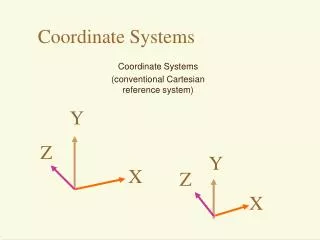
Introduction • Same coordinate system is used on a same “View” of ArcView or same “Data Frame” in ArcMap. • Projection - converting digital map from longitude/latitude to two-dimension coordinate system. • Re-projection - converting from one coordinate system to another
Size and Shape of the Earth • Shape of the Earth is called “geoid” • The sciences of earth measurement is called “Geodesy” • “ellipsoid” - reference to the Earth shape. b=semiminor axis (polar radius) f = (a-b)/a - flattening 1/298.26 for GRS1980, and 1/294.98 for Clarke 1866 a = semimajor axis (equatorial radius) The geoid bulges at the North Pole and is depressed at the South Pole
Geographic Grid • The location reference system for spatial features on the Earth’s surface, consisting of Meridians and Parallels. • Meridians - lines of longitude for E-W direction from Greenwich (Prime Meridian) • Parallels - line of latitude for N-S direction • North and East are positive for lat. and long. such as Cookeville is in (-85.51, 36.17).
DMS and DD (sexagesimal scale) • Longitude/Latitude can be measured in DMS or DD, • For example in downtown Cookeville, a point with (-85.51, 36.17) which is in DD. To convert DD to DMS, we will have to do several steps: for example, to convert -85.51 to DMS, • 0.51 * 60 = 30.6, this add 30 to minute and leave 0.6. • 0.6 * 60 = 36, this add 36 to seconds. Thus, the longitude is (-85o30’36”)
Exercise - convert New York City’s DMS to DD • New York City’s La Guardia Airport is located at (73o54’,40o46’). Convert this DMS to DD.
Exercise 1 - convert New York City’s DMS to DD • New York City’s La Guardia Airport is located at (73o54’,40o46’). Convert this DMS to DD. • 54/60 = 0.9 and 46/60 = 0.77 • (73.90, 40.77) is the answer.
Datum • Spheroid or ellipsoid- a model that approximate the Earth - datum is used to define the relationship between the Earth and the ellipsoid. • Clarke 1866 - was the standard for mapping the U.S. NAD 27 is based on this spheroid, centered at Meades Ranch, Kansas. • WGS84 (GRS80) - from satellite orbital data. More accurate and it is tied into a global network and GPS. NAD 83 is based on this datum. • Horizontal shift between NAD 27 and NAD can be large (fig 2.10) • USGS 7.5 minute quad map is based on NAD 27. • DO NOT MESS UP WITH DATUM!!!!
Exercise 2 • Start “ArcMap” – the program we will use very often in this class. • Add “tn_cnty.shp” from “g:\46505650\Data\1-18-06. • This is an ‘unprojected” shapefile. A shapefile is a layer used in ArcView/ArcGIS consisted of 3 files with extensions “dbf”,”shp”,and ”shx” • “Unprojected” means it is still in DD (or DMS) • Now, find out what datum this layer is based on. (Hint: R-C on tn_cnty.shp select Layer Properties/Sources). However, the true datum is not revealed until you have metadata, or projection information available.
Coordinate Systems • Plane coordinate systems are used in large-scale mapping such as at a scale of 1:24,000. • accuracy in a feature’s absolute position and its relative position to other features is more important than the preserved property of a map projection. • Most commonly used coordinate systems: UTM, UPS, SPC and PLSS
UTM • See the back of front cover for UTM zones. • Divide the world into 60 zones with 6o of longitude each,covering surface between 84oN and 80oS. • Use Transverse Mercator projection with scale factor of 0.9996 at the central meridian. The standard meridian are 180 km east and west of the central meridian. • false origin at the equator and 500,000 meters west of the central meridian in N Hemisphere, and 10,000,000 m south of the equator and 500,000 m west of the central meridian. • Maintain the accuracy of at least one part in 2500 (within one meter accuracy in a 2500 m line)
The SPC System • Developed in 1930. • To maintain required accuracy of one in 10,000, state may have two ore more SPC zones. (see the front side of the back cover) • Transvers Mercator is used for N-S shapes, Lambert conformal conic for E-W direction. • Points in zone are measured in feet origianlly. • State Plane 27 and 83 are two systems. State Plane 83 use GRS80 and meters (instead of feet)
PLSS • Divide state into 6x6 mile squares or townships. Each township was further partitioned into 36 square-mile parcels of 640 acres, called sections • Link for downloading PLSS from Wyoming • http://www.sdvc.uwyo.edu/clearinghouse/howto.html (click on “Browse List > General> Public Land Survey System..>PLSS/Ownership) • Exercise: download a county’s PLSS from Wyoming and load it to the ArcMap or ArcView.
Exercise 3 • Download TIGER Census Data from http://arcdata.esri.com/data/tiger2000/tiger_download.cfm. • Select TN>Putnam and the following data: • Census Tract 2000 • County 2000 • Line Features – Roads • Census Tract Demographics (PL94) • Census Tract Demographics (SF1) • Click {Proceed to Download and Download file} • They come as a zip file. Within this zip file, there are 5 zip files and one readme.html. • Put these files on your own folder (you should create a “1-18” folder within your own folder and store all your data here) • Create a new “Data Frame” and put unzipped layers on this data frame. Rename the Data Frame as “Putnam” • Read the “readme.html” to find out how to obtain metadata of the census data layer. It turns out this
Define the projection(why?) • Define tgr47141lKA,tgr47141cty00, and tgr47141trt00 as “NAD 1983” using ArcToolbox|Data Management Tools| Projections and Transformations|Define Projection
Project Layers • Insert a new “Data Frame” and name it as “UTM83” • Within “Projections and Transformations” select “Feature | Project” • Project the above three layers to UTM 1983NAD. • After you click on the “ Select” from “Spatial Reference Properties”, choose “Projected Coordinate Systems” then “UTM”, “Nad 1983”. • Select “NAD 1983 UTM Zone 16N.prj” from the list. • Remember to check the output dataset name. You may want to change it to “tgr47141cty00_utm83.shp” to reflect the coordinate system. • Use “Batch Project” instead of “Project” to project two layers in one time.
Layout • Use layout to confirm the difference between UTM83 and DD • Switch from “data view” to “layout view” • Overlay Putnam county border maps and see the difference.