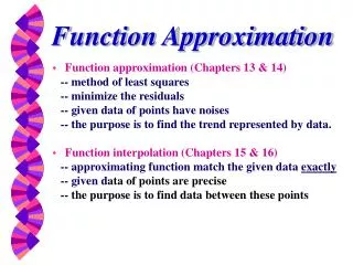
Function Approximation
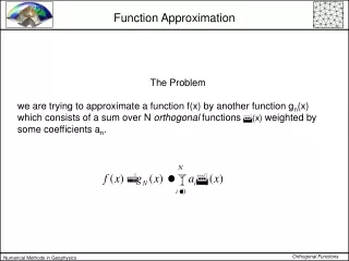
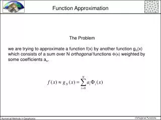
Function Approximation. The Problem we are trying to approximate a function f(x) by another function g n (x) which consists of a sum over N orthogonal functions F (x) weighted by some coefficients a n . The Problem.

Function Approximation
E N D
Presentation Transcript
Function Approximation The Problem we are trying to approximate a function f(x) by another function gn(x) which consists of a sum over N orthogonal functions F(x) weighted by some coefficients an.
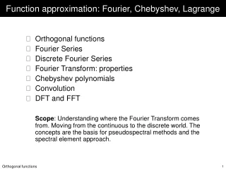
The Problem ... and we are looking for optimal functions in a least squares (l2) sense ... ... a good choice for the basis functions F(x) are orthogonal functions. What are orthogonal functions? Two functions f and g are said to be orthogonal in the interval [a,b] if How is this related to the more conceivable concept of orthogonal vectors? Let us look at the original definition of integrals:
Orthogonal Functions - Definition ... where x0=a and xN=b, and xi-xi-1=x ... If we interpret f(xi) and g(xi) as the ith components of an N component vector, then this sum corresponds directly to a scalar product of vectors. The vanishing of the scalar product is the condition for orthogonality of vectors (or functions). gi fi
Periodic functions Let us assume we have a piecewise continuous function of the form ... we want to approximate this function with a linear combination of 2 periodic functions:
Orthogonality of Periodic functions ... are these functions orthogonal ? ... YES, and these relations are valid for any interval of length 2. Now we know that this is an orthogonal basis, but how can we obtain the coefficients for the basis functions? from minimising f(x)-g(x)
Fourier coefficients optimal functions g(x) are given if ... with the definition of g(x) we get ... leading to
Fourier approximation of |x| ... Example ... leads to the Fourier Serie .. and for n<4 g(x) looks like
Fourier approximation of x2 ... another Example ... leads to the Fourier Serie .. and for N<11, g(x) looks like
Fourier - discrete functions ... what happens if we know our function f(x) only at the points it turns out that in this particular case the coefficients are given by .. the so-defined Fourier polynomial is the unique interpolating function to the function f(xj) with N=2m
Fourier - collocation points ... with the important property that ... ... in our previous examples ... f(x)=|x| => f(x) - blue ; g(x) - red; xi - ‘+’
Fourier series - convergence f(x)=x2 => f(x) - blue ; g(x) - red; xi - ‘+’
Fourier series - convergence f(x)=x2 => f(x) - blue ; g(x) - red; xi - ‘+’
Orthogonal functions - Gibb’s phenomenon f(x)=x2 => f(x) - blue ; g(x) - red; xi - ‘+’ The overshoot for equi-spaced Fourier interpolations is 14% of the step height.
Chebyshev polynomials We have seen that Fourier series are excellent for interpolating (and differentiating) periodic functions defined on a regularly spaced grid. In many circumstances physical phenomena which are not periodic (in space) and occur in a limitedarea. This quest leads to the use of Chebyshev polynomials. We depart by observing that cos(n) can be expressed by a polynomial in cos(): ... which leads us to the definition:
Chebyshev polynomials - definition ... for the Chebyshev polynomials Tn(x). Note that because of x=cos() they are defined in the interval [-1,1] (which - however - can be extended to ).The first polynomials are
Chebyshev polynomials - Graphical The first ten polynomials look like [0, -1] The n-th polynomial has extrema with values 1 or -1 at
Chebyshev collocation points These extrema are not equidistant (like the Fourier extrema) k x(k)
Chebyshev polynomials - interpolation ... we are now faced with the same problem as with the Fourier series. We want to approximate a function f(x), this time not a periodical function but a function which is defined between [-1,1]. We are looking for gn(x) ... and we are faced with the problem, how we can determine the coefficients ck. Again we obtain this by finding the extremum (minimum)
Chebyshev polynomials - interpolation ... to obtain ... ... surprisingly these coefficients can be calculated with FFT techniques, noting that ... and the fact that f(cos) is a 2-periodic function ... ... which means that the coefficients ck are the Fourier coefficients ak of the periodic function F()=f(cos )!
Chebyshev - discrete functions ... what happens if we know our function f(x) only at the points in this particular case the coefficients are given by ... leading to the polynomial ... ... with the property
Chebyshev - collocation points - |x| f(x)=|x| => f(x) - blue ; gn(x) - red; xi - ‘+’ 8 points 16 points
Chebyshev - collocation points - |x| f(x)=|x| => f(x) - blue ; gn(x) - red; xi - ‘+’ 32 points 128 points
Chebyshev - collocation points - x2 f(x)=x2 => f(x) - blue ; gn(x) - red; xi - ‘+’ 8 points The interpolating function gn(x) was shifted by a small amount to be visible at all! 64 points
Chebyshev vs. Fourier - numerical Chebyshev Fourier f(x)=x2 => f(x) - blue ; gN(x) - red; xi - ‘+’ This graph speaks for itself ! Gibb’s phenomenon with Chebyshev?
Chebyshev vs. Fourier - Gibb’s Chebyshev Fourier f(x)=sign(x-) => f(x) - blue ; gN(x) - red; xi - ‘+’ Gibb’s phenomenon with Chebyshev? YES!
Chebyshev vs. Fourier - Gibb’s Chebyshev Fourier f(x)=sign(x-) => f(x) - blue ; gN(x) - red; xi - ‘+’
Fourier vs. Chebyshev Chebyshev Fourier collocation points limited area [-1,1] periodic functions domain basis functions interpolating function
Fourier vs. Chebyshev (cont’d) Chebyshev Fourier coefficients • Gibb’s phenomenon for discontinuous functions • Efficient calculation via FFT • infinite domain through periodicity • limited area calculations • grid densification at boundaries • coefficients via FFT • excellent convergence at boundaries • Gibb’s phenomenon some properties